Factorial ANOVA I

The (fake) dataset for this week is roughly based on a study examining social judgments of job applicants with disabilities: Louvet, E. (2007). Social judgment toward job applicants with disabilities: Perception of personal qualities and competences. Rehabilitation Psychology, 52(3), 297.

The researchers hypothesized that job applicants with disabilities would be rated more negatively with respect to their suitability for a job that required contact with the public compared to a job requiring no public contact. They also hypothesized that applicants with disabilities would be rated more negatively overall compared to participants without a disability. Finally, for the applicants without a disability, they did not expect to find any differences between ratings for contact versus no contact.

The study design was fully between subjects, and all participants were randomly assigned to one of the four conditions.

1. What are the independent variables? What is the dependent variable? What are the three primary questions we can answer with this dataset?

2x2 Factorial ANOVA

A 2x2 between subjects factorial design occurs when you have two independent variables, each with two levels, that have been crossed (4 conditions). Each participant is assigned to ONE of the four conditions. In this example, the researcher manipulated two variables: disability status (no disability versus disability), and job type (requiring public contact). The appropriate analysis for the data is a 2x2 between subject ANOVA.

Begin by importing the dataset. The file to use for this exercise is disability.csv.

disability_data <- read_csv("disability.csv")  #change to where you have the file saved

Data Screening

1. Check that your data imported correctly, and factor any variables that should be factored (if they did not import as factors). Then run descriptives, frequencies, histograms and boxplots by condition to confirm that your data look ready for analysis.

Let’s get started and do some data screening and cleaning!

summary(disability_data)

##      subnum            age         disability          jobtype         
##  Min.   :  1.00   Min.   :18.00   Length:100         Length:100        
##  1st Qu.: 25.75   1st Qu.:20.75   Class :character   Class :character  
##  Median : 50.50   Median :23.00   Mode  :character   Mode  :character  
##  Mean   : 50.50   Mean   :22.52                                        
##  3rd Qu.: 75.25   3rd Qu.:25.00                                        
##  Max.   :100.00   Max.   :26.00                                        
##      rating       race_ethn              GPA           Major          
##  Min.   : 3.00   Length:100         Min.   :1.040   Length:100        
##  1st Qu.: 6.00   Class :character   1st Qu.:2.050   Class :character  
##  Median : 8.00   Mode  :character   Median :2.655   Mode  :character  
##  Mean   : 8.42                      Mean   :2.622                     
##  3rd Qu.:10.00                      3rd Qu.:3.105                     
##  Max.   :15.00                      Max.   :4.000

disability_data<- disability_data %>%
  mutate(disability = factor(disability, 
                             levels = c("disability", "no disability"),
                             labels = c("Disability", "No Disability")),
         race_ethn = as.factor(race_ethn),
         Major = as.factor(Major),
         jobtype = factor(jobtype, 
                          levels = c("no public contact" , "public contact"), 
                          labels = c("No Public Contact" , "Public Contact")))

disability_data %>%
  group_by(disability, jobtype) %>%
  summarize(mean = mean(rating, na.rm = TRUE),
            sd = sd(rating, na.rm= TRUE),
            min = min(rating, na.rm = TRUE),
            max = max(rating, na.rm = TRUE))

## # A tibble: 4 x 6
## # Groups:   disability [2]
##   disability    jobtype            mean    sd   min   max
##   <fct>         <fct>             <dbl> <dbl> <dbl> <dbl>
## 1 Disability    No Public Contact  8.44  3.25     5    15
## 2 Disability    Public Contact     6.36  1.91     3     9
## 3 No Disability No Public Contact  9.56  2.89     4    15
## 4 No Disability Public Contact     9.32  2.10     6    13

ggplot(disability_data, aes(x = rating, fill = jobtype)) +
  geom_histogram(bins = 12) +
  facet_wrap(~disability)

qplot(y = rating, x = disability, fill = jobtype, data = disability_data, 
      geom = "boxplot") 

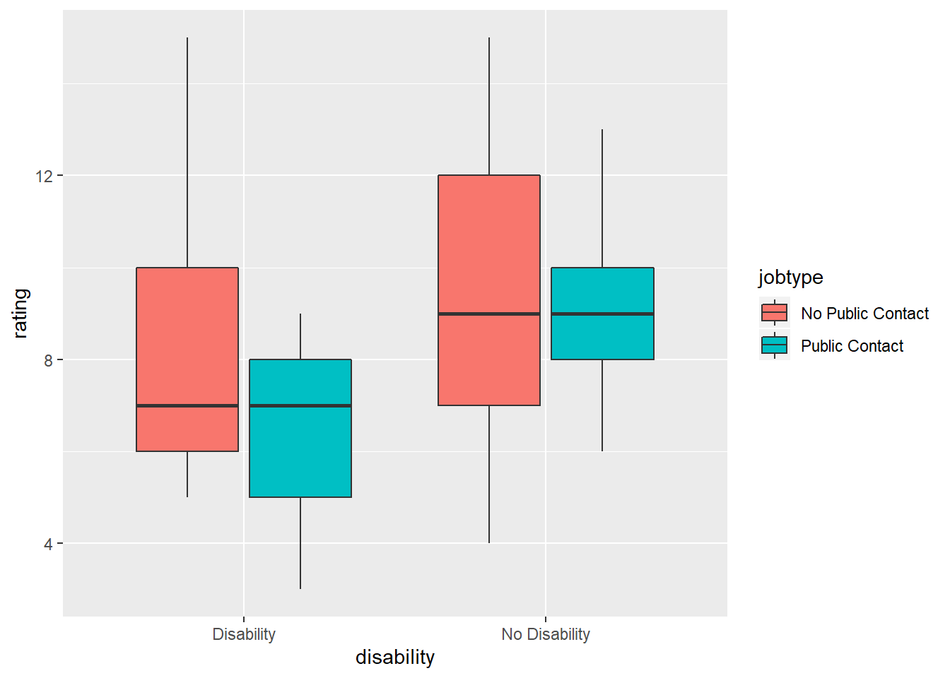In the code above, we first looked at some basic summary statistics using the summary function. Then, we factored our independent variables, jobtype and disability. Then we ran some descriptive statistics, breaking down the groups by both factors. Finally, we plotted a histogram and boxplot.

Running the Factorial ANOVA

Now we are ready to run the ANOVA. We’ll use the ez package again like we did with the one-way ANOVA. We have two between subjects variables now–disability and jobtype. We will enter both of these variables togeter on the the between line. We will need to enter the variable names using a .(IV1, IV2) format. Remember that we enter the dependent variable on the dv line, and wid is the subject or participant number. type=3 gives us Type III sum of squares, and detailed=T will give us the sum of squares values. The results of the ANOVA are saved to an object called model. Use print(model) to see the results.

Another way to print the results in a better looking table is to use the apaTables package. Within that package, there is a function called apa.ezANOVA.table that will print the results of the ANOVA model in a neatly formatted table. You can save the table as a word document to your working directory (the default location).

options(scipen=999)  #turns off scientific notation
library(ez)  #library needed for the ezANOVA function

model <- ezANOVA(data = disability_data,
        dv = rating,
        between = .(disability, jobtype),
        wid = subnum,
        type = 3,
        detailed = T,
        return_aov = T)

print(model)

## $ANOVA
##               Effect DFn DFd     SSn    SSd           F
## 1        (Intercept)   1  96 7089.64 647.52 1051.095626
## 2         disability   1  96  104.04 647.52   15.424759
## 3            jobtype   1  96   33.64 647.52    4.987398
## 4 disability:jobtype   1  96   21.16 647.52    3.137139
##                                                               p p<.05
## 1 0.00000000000000000000000000000000000000000000000000001646211     *
## 2 0.00016170639391939218166421854405712110747117549180984497070     *
## 3 0.02785509025523449228023409318666381295770406723022460937500     *
## 4 0.07970154348101042562912965649957186542451381683349609375000      
##          ges
## 1 0.91631038
## 2 0.13843206
## 3 0.04938634
## 4 0.03164443
## 
## $`Levene's Test for Homogeneity of Variance`
##   DFn DFd   SSn    SSd        F         p p<.05
## 1   3  96 17.72 294.24 1.927134 0.1303328      
## 
## $aov
## Call:
##    aov(formula = formula(aov_formula), data = data)
## 
## Terms:
##                 disability jobtype disability:jobtype Residuals
## Sum of Squares      104.04   33.64              21.16    647.52
## Deg. of Freedom          1       1                  1        96
## 
## Residual standard error: 2.597114
## Estimated effects may be unbalanced

We can use the apaTables package to print the results into a formatted table in a Word document:

library(apaTables)
apa.ezANOVA.table(model, file="ANOVA Results Table.doc") #saves table of results to word doc

## 
## 
## ANOVA results
##  
## 
##             Predictor df_num df_den  SS_num SS_den       F    p ges
##           (Intercept)      1     96 7089.64 647.52 1051.10 .000 .92
##            disability      1     96  104.04 647.52   15.42 .000 .14
##               jobtype      1     96   33.64 647.52    4.99 .028 .05
##  disability x jobtype      1     96   21.16 647.52    3.14 .080 .03
## 
## Note. df_num indicates degrees of freedom numerator. df_den indicates degrees of freedom denominator. 
## SS_num indicates sum of squares numerator. SS_den indicates sum of squares denominator. 
## ges indicates generalized eta-squared.
## 

A Note on Sum of Squares

The ezANOVA code above contains the line type=3, which will then esimate the model use Type III Sums of Squares. What are Type III Sums of Squares? There are actually 3 “Types” of sums of squares. The default in R is Type I, but the default in other statistical programs like SPSS and SAS is Type III. Field gives a brief description of each of the types in Ch 11 (Jane SuperBrain 11.1, pgs 475-476). The very short version of the story is that for Type I SS, order of entry of the variables matters when the variability is being partitioned. In Type III, order doesn’t matter. Type III is better for unbalanced designs, and both the main effects and interactions are interpretable and meaningful (although in most cases, if you have a significant interaction, it supercedes the main effects). We will stick with Type III for this course, but know if you google this issue, you will find a raging debate between statisticians about what type of SS is best!

Post-hoc Analyses and Graphing the Means

When you have a significant interaction in a 2x2 between subjects design, you do not need to do post-hoc tests on the main effects. This is because you only have two levels–if the main effect is significant, the means are significantly different from one other. Look at the means to see which group is significantly higher (or lower).

With a significant interaction, you should just describe the nature of the interaction (i.e., The difference between the control and experimental condition was larger for men than it was for women). With more complex factorial designs, you will need to do simple effects analyses to determine the nature of the interaction. We’ll get to that next week!

Plot the Means

One of the best ways to begin to unpack and understand an interaction is to graph the means.

1. Use ggplot2 to create a bar graph with error bars. Label the axes, and use the cleanup code to print a publication-quality graph.
   

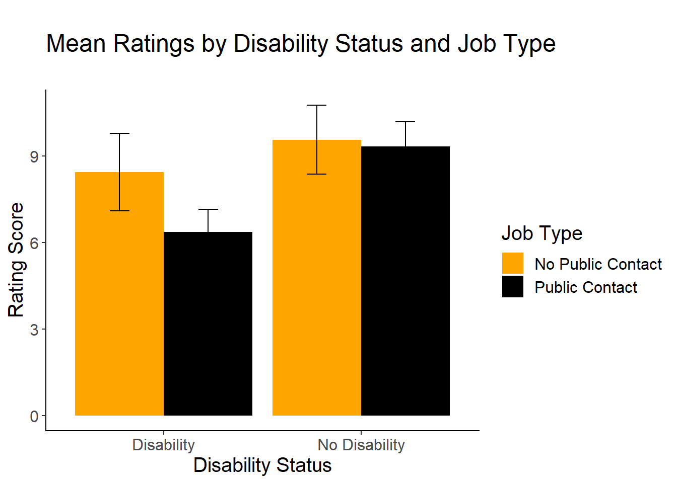
Here is how to plot a bar graph of our means by condition:

cleanup = theme(panel.grid.major = element_blank(), 
                panel.grid.minor = element_blank(), 
                panel.background = element_blank(), 
                axis.line.x = element_line(color = "black"),
                axis.line.y = element_line(color = "black"),
                legend.key = element_rect(fill = "white"),
                text = element_text(size = 15))
#clean-up code makes the graph publication-ready; you don't need it if you don't want it

bargraph = ggplot(disability_data, aes(x = disability, y=rating, fill=jobtype))
bargraph +
  stat_summary(fun.y = mean,
               geom = "bar",                
               position="dodge") +
  stat_summary(fun.data = mean_cl_normal, 
               geom = "errorbar",
               position = position_dodge(width = 0.90),
               width = .2) +
  xlab("Disability Status") +
  ylab("Rating Score") +
  scale_fill_manual(values = c("orange", "black"), name= "Job Type")+
  cleanup +
  ggtitle("\nMean Ratings by Disability Status and Job Type\n")

Effect Size

The ezANOVA output includes an effect size measure for the main effects and the interaction.But remember with ANOVA, we are often interested in the standardized difference between the means (i.e., Cohen’s d) instead of the percentage of variablity accounted for.

1. Use MOTE to calculate cohen’s d for the two significant main effects.
   

For the interaction, we’ll need to split the data and look at two different comparisons: no public versus public for the Disability condition, and no public versus public for the No Disability condition. Here we will start with splitting the data into the two separate files.

No.Disability.Group<- disability_data %>%
  dplyr::filter(disability == "No Disability")

Disability.Group<- disability_data %>%
  dplyr::filter(disability == "Disability")

Then we can run t-tests separately in each dataset to see if there are significant differences between the groups within each disability group.

t.test(rating~jobtype, 
       data=No.Disability.Group, 
       var.equal=TRUE)

## 
## 	Two Sample t-test
## 
## data:  rating by jobtype
## t = 0.33629, df = 48, p-value = 0.7381
## alternative hypothesis: true difference in means is not equal to 0
## 95 percent confidence interval:
##  -1.194942  1.674942
## sample estimates:
## mean in group No Public Contact    mean in group Public Contact 
##                            9.56                            9.32

t.test(rating~jobtype,
       data=Disability.Group,
       var.equal=TRUE)

## 
## 	Two Sample t-test
## 
## data:  rating by jobtype
## t = 2.7553, df = 48, p-value = 0.008261
## alternative hypothesis: true difference in means is not equal to 0
## 95 percent confidence interval:
##  0.5621816 3.5978184
## sample estimates:
## mean in group No Public Contact    mean in group Public Contact 
##                            8.44                            6.36

The last step is to calculate effect sizes for each comparison. Here, I’ll use favstats to get the descriptive statistics for each condition, and then use the MOTE package to calculate Cohen’s D for each comparison.

favstats(rating~jobtype, data=No.Disability.Group)

##             jobtype min Q1 median Q3 max mean       sd  n missing
## 1 No Public Contact   4  7      9 12  15 9.56 2.887906 25       0
## 2    Public Contact   6  8      9 10  13 9.32 2.096028 25       0

favstats(rating~jobtype, data=Disability.Group)

##             jobtype min Q1 median Q3 max mean       sd  n missing
## 1 No Public Contact   5  6      7 10  15 8.44 3.254228 25       0
## 2    Public Contact   3  5      7  8   9 6.36 1.912241 25       0

library(MOTE)
d.nodissgroup <- d.ind.t(9.56, 9.32, 2.88, 2.09, 25, 25)
d.disabilitygroup <- d.ind.t(8.44, 6.36, 3.25, 1.91, 25, 25)

d.nodissgroup$estimate  

## [1] "$d_s$ = 0.10, 95\\% CI [-0.46, 0.65]"

d.disabilitygroup$estimate

## [1] "$d_s$ = 0.78, 95\\% CI [0.20, 1.35]"

Writing up the Results

To determine if disability status affected ratings of suitability for job based on whether that job required contact with the public, we conducted a 2 (disability group: disability versus no disability) by 2 (job type: contact versus no contact) between subjects factorial ANOVA. Levene’s test was not statistically significant, F(3,96) = 1.93, p = .13. The main effect of disability status was statistically significant, F(1, 96) = 15.42, p< .001, ${\eta }^2$ = .14. The main effect of job type was also statstically significant, F(1, 96) = 4.99, p.028, ${\eta }^2$ = .05. The interaction between disability status and job type was marginally significant, F(1, 96) = 3.14, p.080, ${\eta }^2$ = .03.

Figure 1 contains the means and standard error bars as a function of both disability status and job type. Overall, job applicants wihtout a disability were rated higher than applicants with a disability, and applicants were rated higher for the no contact job compared to the contact job. However, when looking within each disability condition, the difference between ratings based on job type is greater($d_s$ = 0.78, 95\% CI [0.20, 1.35]) in the disability condition compared to the no disability condition ($d_s$ = 0.10, 95\% CI [-0.46, 0.65]).