Factorial ANOVA II

Thus far, you have learned how to conduct a one-way and simple 2-way (2x2) between subjects ANOVA using R. We can use ANOVA for more complex designs that involved more than 2 levels per independent variable (3 or more conditions), and more than 2 independent variables. However, I don’t recommend designing a study with more than 3 independent variables. Three IVs can be challenging enough! For this lab exercise, we will work through a 2 x 3 ANOVA using a dataset from Field.

2 x 3 Factorial ANOVA

From Field pg. 501: An anthropologist was interested in the effects of alcohol on mate selection at nightclubs. She hypothesized that subjective perceptions of attractiveness would become more inaccurate as the amount of alcohol consumed increased. She was also interested in whether the effect would be different for men versus women. She designed a study where 24 male and 24 female students were randomly assigned to drink a non-alcoholic beer (0 pints of alcoholic beer), 2 pints of beer, or 4 pints of beer. At the end of the night, a photograph was taken of the person the participant was chatting with. A pool of independent judges then rated the photographs on attractiveness on a scale of 0-100 (100 = very attractive).

1. What are the independent variables? What is the dependent variable? What are the three primary questions we can answer with this dataset?

Running a Factorial ANOVA

The process and code for running a factorial ANOVA is pretty much identical to the process we followed last week. Begin by importing the dataset, and then go through your (hopefully, by now) routine for cleaning and screening the data.

goggles_data <- read_csv("goggles.csv")

Data Screening

As always, the first step of the analysis should be the clean and screen the data. Do this on your own before looking at the code below.

1. Check that your data imported correctly, and factor any variables that should be factored (if they did not import as factors). Then run descriptives and boxplots by condition to confirm that your data look ready for analysis. Some information you may need to help you factor the variables: Gender was coded 1= female, 0 = male. Alcohol was coded 1 = 0 pints, 2 = 2 pints, 3 = 4 pints.

To clean and screen, we’ll use summary to get some basic stats, factor our IVs, calculate descriptive statistics, and look at histograms and boxplots as a function of our two IVS:

summary(goggles_data)

##      Gender       Alcohol  Attractiveness 
##  Min.   :0.0   Min.   :1   Min.   :20.00  
##  1st Qu.:0.0   1st Qu.:1   1st Qu.:53.75  
##  Median :0.5   Median :2   Median :60.00  
##  Mean   :0.5   Mean   :2   Mean   :58.33  
##  3rd Qu.:1.0   3rd Qu.:3   3rd Qu.:66.25  
##  Max.   :1.0   Max.   :3   Max.   :85.00

goggles_data<- goggles_data %>%
  mutate(Gender = factor(Gender, 
                             levels = c(1,0),
                             labels = c("Female", "Male")),
         Alcohol = factor(Alcohol, 
                          levels = c(1,2,3), 
                          labels = c("None" , "2 Pints", "4 Pints")))

goggles_data %>%
  group_by(Gender, Alcohol) %>%
  summarize(mean = mean(Attractiveness, na.rm = TRUE),
            sd = sd(Attractiveness, na.rm= TRUE),
            min = min(Attractiveness, na.rm = TRUE),
            max = max(Attractiveness, na.rm = TRUE))

## # A tibble: 6 x 6
## # Groups:   Gender [2]
##   Gender Alcohol  mean    sd   min   max
##   <fct>  <fct>   <dbl> <dbl> <dbl> <dbl>
## 1 Female None     60.6  4.96    55    70
## 2 Female 2 Pints  62.5  6.55    50    70
## 3 Female 4 Pints  57.5  7.07    50    70
## 4 Male   None     66.9 10.3     50    80
## 5 Male   2 Pints  66.9 12.5     45    85
## 6 Male   4 Pints  35.6 10.8     20    55

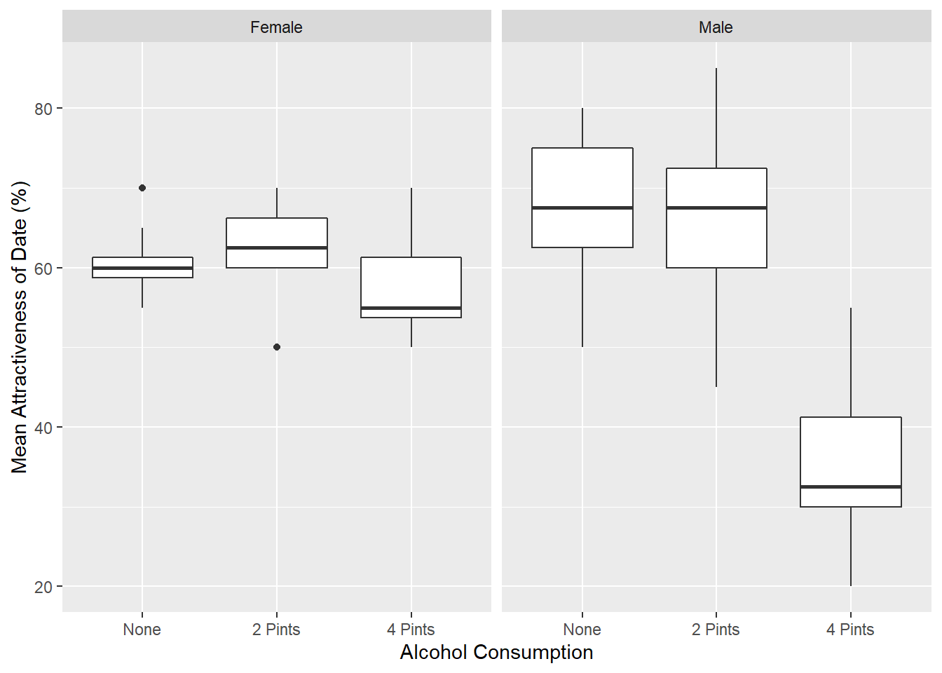
boxplot <- ggplot(goggles_data, aes(Alcohol, Attractiveness))
boxplot + 
  geom_boxplot() + 
  facet_wrap(~Gender) + 
  labs(x = "Alcohol Consumption", y = "Mean Attractiveness of Date (%)")

Running the Analyaiss

We’ll use the ez package to run the factorial ANOVA. To use ezANOVA we need to first add a subject number to our dataset.

goggles_data$partno <-1:nrow(goggles_data)

Double-check that a new variable has been added to the dataset (there should now be 4 variables). If everything looks good, you can move on to running the ANOVA.

We have two between subjects variables–Gender and Alcohol. We will enter both of these variables togeter on the the between line. Remember from last week that you’ll need to enter the variable names using a .(IV1, IV2) format. Save the results of the model to an object called goggles.model and then print the results using the print function (to get the ANOVA results and Levene’s Test), as well as the apa.ezANOVA.table function from apaTables.

options(scipen=999)  #turns off scientific notation

library(ez)
options(contrasts = c("contr.sum", "contr.poly"))
goggles.model <- ezANOVA(data = goggles_data,
        dv = Attractiveness,
        between = .(Gender, Alcohol),
        wid = partno,
        type = 3,
        detailed = T,
        return_aov = T)

print(goggles.model)

## $ANOVA
##           Effect DFn DFd        SSn    SSd           F
## 1    (Intercept)   1  42 163333.333 3487.5 1967.025090
## 2         Gender   1  42    168.750 3487.5    2.032258
## 3        Alcohol   2  42   3332.292 3487.5   20.065412
## 4 Gender:Alcohol   2  42   1978.125 3487.5   11.911290
##                                               p p<.05        ges
## 1 0.0000000000000000000000000000000000006571285     * 0.97909434
## 2 0.1613818326039029027452187392555060796439648       0.04615385
## 3 0.0000007649010839806060044632901595562657349     * 0.48862074
## 4 0.0000798660282763287448669006773904754936666     * 0.36192110
## 
## $`Levene's Test for Homogeneity of Variance`
##   DFn DFd      SSn    SSd        F         p p<.05
## 1   5  42 235.4167 1387.5 1.425225 0.2350678      
## 
## $aov
## Call:
##    aov(formula = formula(aov_formula), data = data)
## 
## Terms:
##                   Gender  Alcohol Gender:Alcohol Residuals
## Sum of Squares   168.750 3332.292       1978.125  3487.500
## Deg. of Freedom        1        2              2        42
## 
## Residual standard error: 9.112393
## Estimated effects may be unbalanced

library(apaTables)
apa.ezANOVA.table(goggles.model)

## 
## 
## ANOVA results
##  
## 
##         Predictor df_num df_den    SS_num  SS_den       F    p ges
##       (Intercept)      1     42 163333.33 3487.50 1967.03 .000 .98
##            Gender      1     42    168.75 3487.50    2.03 .161 .05
##           Alcohol      2     42   3332.29 3487.50   20.07 .000 .49
##  Gender x Alcohol      2     42   1978.12 3487.50   11.91 .000 .36
## 
## Note. df_num indicates degrees of freedom numerator. df_den indicates degrees of freedom denominator. 
## SS_num indicates sum of squares numerator. SS_den indicates sum of squares denominator. 
## ges indicates generalized eta-squared.
## 

1. Interpret the results of Levene’s Test. Is there homogeneity of variances?

2. Interpret the F-statistics for the main effects and interactions. Are there significant effects?

Post-hocs, Planned Comparisons, and Contrasts

The ANOVA is an omnibus test, and we are often more interested in specific comparsions than in the overall main effects and interaction(s). With more than 2 levels There are a number of ways we can break down main effects and interactions. If we do not have any apriori hypotheses about specific mean differences between conditions or groups, then post-hoc tests are the best way to go. However, if you have specific apriori hypotheses about which means are different, planned comparisons or contrasts are the most appropriate.

Main Effects. If an IV as two levels, there is nothing left to do. With more than 2 levels, post-hoc t-tests can be used to determine which means are statistically significantly different from one another.

Interactions. If the interaction is significant, you have to make a decision about how you want to break it down. For example, we could break down the significant interaction from the goggles study by looking at gender differences within each level of alcohol (compare men and women who drank 0 pints, men and women who drank 2 pints, and men and women who drank 4 pints). Alternatively, we could look at the effects of alcohol within each gender (for men only, compare 0 v 2, 0 v 4, and 2 v 4 for men, and then do the same thing for women only). The former requires 3 tests, while the latter involves 6 tests. So how do you decide which way to go? It depends. Theory should be a consideration. Type I error inflation is also an issue. Fewer tests are better. However, you can always adjust for multiple comparisons (Bonferroni, Holm, etc), so if you have a reason to go the route that requires more tests, go for it.

Post-hoc Tests

Based on the results of the ANOVA, there is a significant main effect of Alcohol and a significant interaction between Gender and Alcohol. We’ll start with breaking down the main effect of Alcohol (keep in mind though that we shouldn’t focus too much on main effects in the presence of an interaction).

There are three Alcohol conditions: 0 pints, 2 pints, and 4 pints. Let’s first graph the means with error bars.

alcohol_graph <- ggplot(goggles_data, aes(Alcohol, Attractiveness))
alcohol_graph + 
  stat_summary(fun.y = mean, geom = "bar", fill = "Light Blue", colour = "Black") + 
  stat_summary(fun.data = mean_cl_normal, geom = "errorbar", position = position_dodge(width = 0.90), width = .2) +
  labs(x = "Alcohol Consumption", y = "Mean Attractiveness of Date (%)") +
  scale_y_continuous(breaks=seq(0,80, by = 10))

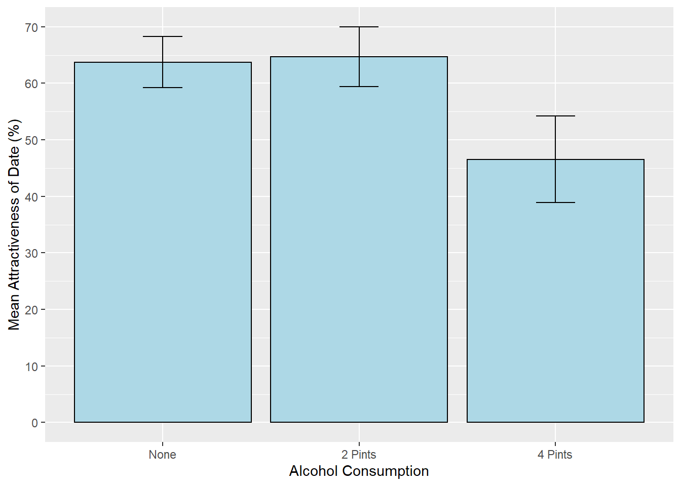
Based on the graph, it looks like the 0 pint and 2 pint conditions are similar, while the 4 pint condition has a lower mean than the other two conditions.

Now, use the pairwise.t.test function to examine differences between the conditions. Note that the means for each of these conditions is calculated by summing across levels of the other independent variable. To adjust for multiple comparisons, use a bonferroni correction (or another correction such as Holm).

pairwise.t.test(goggles_data$Attractiveness, goggles_data$Alcohol, 
                paired = F,
                var.equal = T,
                p.adjust.method = "bonferroni")

## 
## 	Pairwise comparisons using t tests with pooled SD 
## 
## data:  goggles_data$Attractiveness and goggles_data$Alcohol 
## 
##         None    2 Pints
## 2 Pints 1.00000 -      
## 4 Pints 0.00024 0.00011
## 
## P value adjustment method: bonferroni

1. Although the main effect of gender is not significant, plot the means (with error bars) for gender.

Contrasts and Planned Comparisons

The concept of contrasts was introduced a few weeks ago when you learned how to conduct a one-way ANOVA. A contrast is a linear combination of 2 or more means with coefficients that sum to zero.

There are number of interesting contrasts that we could do with this data. For example, we could examine whether any alcohol (combining the 2 and 4 pint groups) is significantly different from the no alcohol group. We could then examine whether 2 pints versus 4 pints are different from one another. To set up these contrasts, we need to assign each group a coefficient. Remember that the contrast coefficients for a particular contrast should sum to 0. In the table below, you can see the coefficients we will need to conduct these two contrasts, and that if you sum across the row, it adds up to 0.

Contrast	0 Pint	2 Pint	4 Pint
Contrast 1: No Alcohol v Alcohol	-2	1	1
Contrast 2: 2 pints v 4 pints	0	-1	1

To set up contrasts in R, we will use contrasts to tell R which comparisons we need. We will set up contrasts for both Alcohol and Gender. Once we set those up, we then need to re-run the ANOVA model. However, instead of using ezANOVA, we’ll need to use another method. The aov function runs the same analysis as ezANOVA with one key difference–aov uses Type I sum of squares. We need Type III. To get around this issue, we will use the Anova function from the car library. If you don’t already have car installed, do that first. Anova is a wrapper function for aov that allows us to request Type III sums of squares.

When you call the output of the aov model, you should get the same results as when you ran it above using ezANOVA. Note that the output does not contain the contrasts we requested. To get the contrast output, we need to use summary.lm(modelname).

library(car)
contrasts(goggles_data$Alcohol)<-cbind(c(-2, 1, 1), c(0, -1, 1))
contrasts(goggles_data$Gender)<-c(-1, 1)

#run the model with aov
goggles_model_withcontrasts<-aov(Attractiveness ~ Gender*Alcohol, data = goggles_data)

#apply the Anova function from the car package to the model results
Anova(goggles_model_withcontrasts, type="III")

## Anova Table (Type III tests)
## 
## Response: Attractiveness
##                Sum Sq Df   F value                Pr(>F)    
## (Intercept)    163333  1 1967.0251 < 0.00000000000000022 ***
## Gender            169  1    2.0323                0.1614    
## Alcohol          3332  2   20.0654          0.0000007649 ***
## Gender:Alcohol   1978  2   11.9113          0.0000798660 ***
## Residuals        3488 42                                    
## ---
## Signif. codes:  0 '***' 0.001 '**' 0.01 '*' 0.05 '.' 0.1 ' ' 1

#print the results
summary.lm(goggles_model_withcontrasts)

## 
## Call:
## aov(formula = Attractiveness ~ Gender * Alcohol, data = goggles_data)
## 
## Residuals:
##     Min      1Q  Median      3Q     Max 
## -21.875  -5.625  -0.625   5.156  19.375 
## 
## Coefficients:
##                  Estimate Std. Error t value             Pr(>|t|)    
## (Intercept)        58.333      1.315  44.351 < 0.0000000000000002 ***
## Gender1            -1.875      1.315  -1.426             0.161382    
## Alcohol1           -2.708      0.930  -2.912             0.005727 ** 
## Alcohol2           -9.062      1.611  -5.626           0.00000137 ***
## Gender1:Alcohol1   -2.500      0.930  -2.688             0.010258 *  
## Gender1:Alcohol2   -6.562      1.611  -4.074             0.000201 ***
## ---
## Signif. codes:  0 '***' 0.001 '**' 0.01 '*' 0.05 '.' 0.1 ' ' 1
## 
## Residual standard error: 9.112 on 42 degrees of freedom
## Multiple R-squared:  0.6111,	Adjusted R-squared:  0.5648 
## F-statistic:  13.2 on 5 and 42 DF,  p-value: 0.00000009609

Field gives a nice walk-through of interpreting the output from the contrasts on page 524, so I won’t repeat it here.

Simple Effects

As mentioned above, when you have a significant interaction, you need to break it down to figure out the exact nature of that interaction. You have several options for how to do that, and the method you select should hopefully be driven by your hypotheses. With the beer googles example, the researcher was interested in whether the effect of alcohol was the same for men and women. To understand the nature of the interaction, we need to use Simpe Effects Analyses. Although it called simple, running these analyses can be a bit tricky.

You can follow the instructions that Field provides on page 526-528. With that method, you create a new variable in the dataset called simple that combines all of the independent variables into one variable with the number of levels equal to IV#1 x IV#2 (so in this case, 2 x 3 = 6 levels). Then you set up the contrasts, run a regression model, and then get the output for the contrasts.

#simple effects--Field (pg 526-528)
goggles_data$simple<-gl(6,8)
goggles_data$simple<-factor(goggles_data$simple, 
                           levels = c(1:6), 
                           labels = c("F_None","F_2pints", "F_4pints","M_None","M_2pints", "M_4pints"))

alcEffect1<-c(-2, 1, 1, -2, 1, 1)
alcEffect2<-c(0, -1, 1, 0, -1, 1)
gender_none<-c(-1, 0, 0, 1, 0, 0)
gender_twoPint<-c(0, -1, 0, 0, 1, 0)
gender_fourPint<-c(0, 0, -1, 0, 0, 1)
simpleEff<-cbind(alcEffect1, alcEffect2, gender_none, gender_twoPint, gender_fourPint)

contrasts(goggles_data$simple)<-simpleEff
simpleEffectModel<-aov(Attractiveness ~ simple, data = goggles_data)
summary.lm(simpleEffectModel)

## 
## Call:
## aov(formula = Attractiveness ~ simple, data = goggles_data)
## 
## Residuals:
##     Min      1Q  Median      3Q     Max 
## -21.875  -5.625  -0.625   5.156  19.375 
## 
## Coefficients:
##                       Estimate Std. Error t value             Pr(>|t|)    
## (Intercept)             58.333      1.315  44.351 < 0.0000000000000002 ***
## simplealcEffect1        -2.708      0.930  -2.912              0.00573 ** 
## simplealcEffect2        -9.062      1.611  -5.626           0.00000137 ***
## simplegender_none        3.125      2.278   1.372              0.17742    
## simplegender_twoPint     2.188      2.278   0.960              0.34243    
## simplegender_fourPint  -10.938      2.278  -4.801           0.00002025 ***
## ---
## Signif. codes:  0 '***' 0.001 '**' 0.01 '*' 0.05 '.' 0.1 ' ' 1
## 
## Residual standard error: 9.112 on 42 degrees of freedom
## Multiple R-squared:  0.6111,	Adjusted R-squared:  0.5648 
## F-statistic:  13.2 on 5 and 42 DF,  p-value: 0.00000009609

An alternative, and less intense, strategy is to subset or filter the data based on the levels of one of the independent variables, and then conduct t-tests comparing levels of the other IV within each of the levels of the other IV. We’ll need to do the alpha correction manually. Since we are doing three t-tests, we can divide alpha by 3, .05/3 = .017. Any p-value less than .017 will be considered statistically significant.

goggles_data %>% 
  dplyr::filter(Alcohol == "None") %>%
  t.test(Attractiveness~Gender, data=., var.equal=TRUE)

## 
## 	Two Sample t-test
## 
## data:  Attractiveness by Gender
## t = -1.543, df = 14, p-value = 0.1451
## alternative hypothesis: true difference in means is not equal to 0
## 95 percent confidence interval:
##  -14.937379   2.437379
## sample estimates:
## mean in group Female   mean in group Male 
##               60.625               66.875

goggles_data %>% 
  dplyr::filter(Alcohol == "2 Pints") %>%
  t.test(Attractiveness~Gender, data=., var.equal=TRUE)

## 
## 	Two Sample t-test
## 
## data:  Attractiveness by Gender
## t = -0.87598, df = 14, p-value = 0.3958
## alternative hypothesis: true difference in means is not equal to 0
## 95 percent confidence interval:
##  -15.086958   6.336958
## sample estimates:
## mean in group Female   mean in group Male 
##               62.500               66.875

goggles_data %>% 
  dplyr::filter(Alcohol == "4 Pints") %>%
  t.test(Attractiveness~Gender, data=., var.equal=TRUE)

## 
## 	Two Sample t-test
## 
## data:  Attractiveness by Gender
## t = 4.7819, df = 14, p-value = 0.0002923
## alternative hypothesis: true difference in means is not equal to 0
## 95 percent confidence interval:
##  12.06361 31.68639
## sample estimates:
## mean in group Female   mean in group Male 
##               57.500               35.625

Given what you know about R at this point, you might be thinking, “Hasn’t someone come up with a package to make doing simple effects analyses easier?” The answer is YES! The emmeans package can calculate comparisons/contrasts for main effects and interactions. You should send some time looking through and reading the vignettes for the package, especially if you think you might be using factorial ANOVAs in your future research. The code below will print out the marginal means with standard errors, as wel as pairwise contrasts of gender at each level of alcohol (equivalent to what we did above).

The default p-value adjustment for emmeans is Tukey. However, emmeans applies this for each family of tests. In this example, we have three families of tests (the three levels of alcohol). Because we only have one test per family, there is no p-value adjustment applied. If you have more than one comparison per family, you would get an adjusted p-value.

library(emmeans)
emmeans(goggles.model$aov, pairwise~Gender|Alcohol)

## $emmeans
## Alcohol = None:
##  Gender emmean   SE df lower.CL upper.CL
##  Female   60.6 3.22 42     54.1     67.1
##  Male     66.9 3.22 42     60.4     73.4
## 
## Alcohol = 2 Pints:
##  Gender emmean   SE df lower.CL upper.CL
##  Female   62.5 3.22 42     56.0     69.0
##  Male     66.9 3.22 42     60.4     73.4
## 
## Alcohol = 4 Pints:
##  Gender emmean   SE df lower.CL upper.CL
##  Female   57.5 3.22 42     51.0     64.0
##  Male     35.6 3.22 42     29.1     42.1
## 
## Confidence level used: 0.95 
## 
## $contrasts
## Alcohol = None:
##  contrast      estimate   SE df t.ratio p.value
##  Female - Male    -6.25 4.56 42 -1.372  0.1774 
## 
## Alcohol = 2 Pints:
##  contrast      estimate   SE df t.ratio p.value
##  Female - Male    -4.38 4.56 42 -0.960  0.3424 
## 
## Alcohol = 4 Pints:
##  contrast      estimate   SE df t.ratio p.value
##  Female - Male    21.88 4.56 42  4.801  <.0001

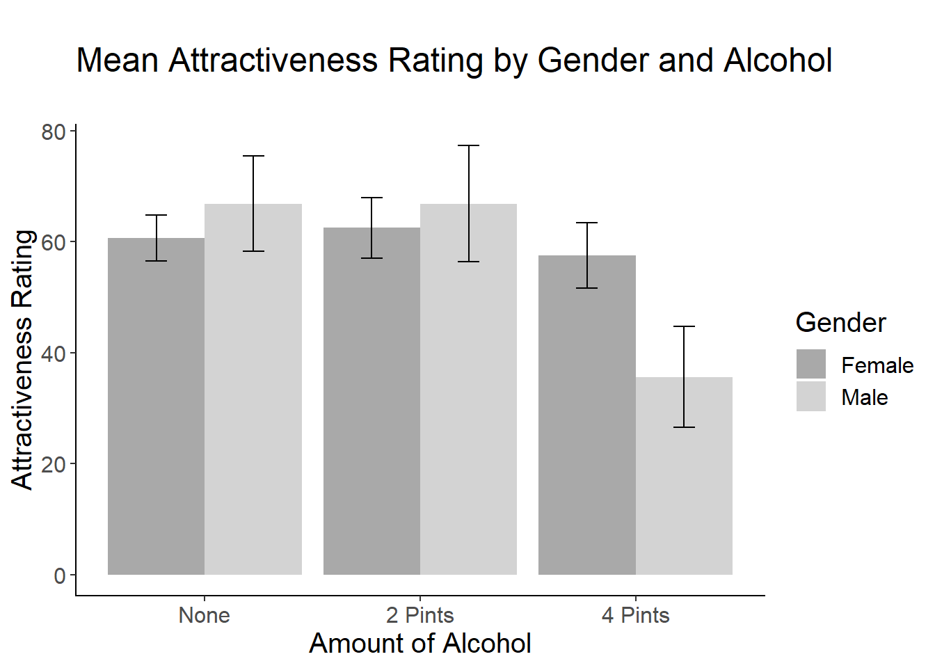
Graphing the Interaction

Now let’s create a bar plot of the means (and error bars) as a function of both alcohol and gender. Use the cleanup code to make it publication-quality.

cleanup = theme(panel.grid.major = element_blank(), 
                panel.grid.minor = element_blank(), 
                panel.background = element_blank(), 
                axis.line.x = element_line(color = "black"),
                axis.line.y = element_line(color = "black"),
                legend.key = element_rect(fill = "white"),
                text = element_text(size = 15))

bargraph = ggplot(goggles_data, aes(x = Alcohol, y=Attractiveness, fill=Gender))
bargraph +
  stat_summary(fun.y = mean,
               geom = "bar",                
               position="dodge") +
  stat_summary(fun.data = mean_cl_normal, 
               geom = "errorbar",
               position = position_dodge(width = 0.90),
               width = .2) +
  xlab("Amount of Alcohol") +
  ylab("Attractiveness Rating") +
  scale_fill_manual(values = c("dark gray", "light gray"), name= "Gender")+
  ggtitle("\nMean Attractiveness Rating by Gender and Alcohol\n")+
  cleanup

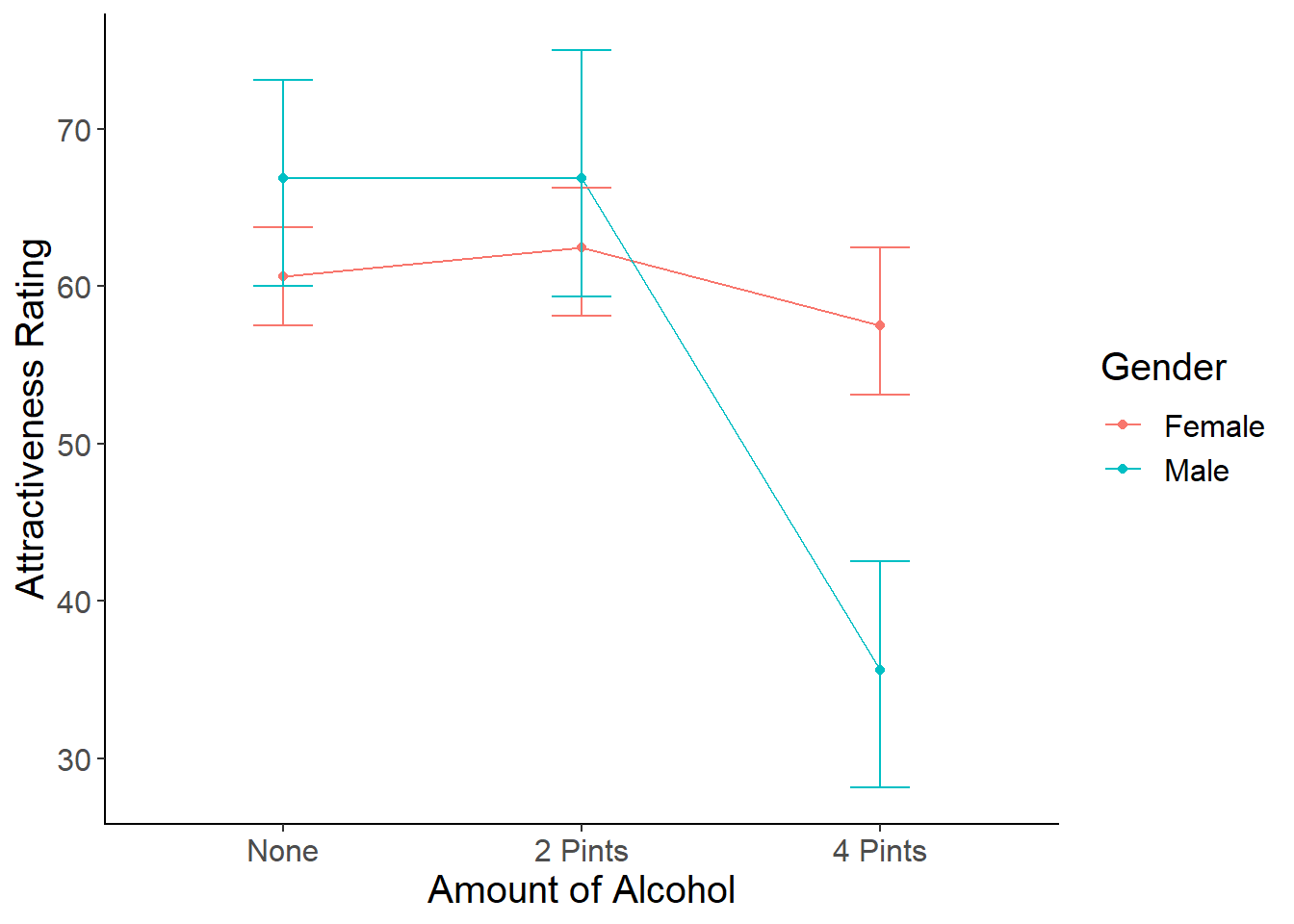
1. Field uses a line graph to display the interaction. Using what you know about ggplot (and Google, if you need it), create a line graph that shows the interaction. Include the error bars.

Here is my version of the line graph:

#Line Graph
linegraph <- ggplot(goggles_data, aes(x = Alcohol, y=Attractiveness, color=Gender)) +
  stat_summary(fun.y = mean,
               geom = "point") +
  stat_summary(fun.y = mean, 
               geom = "line", aes(group= Gender)) + 
  stat_summary(fun.data = mean_cl_boot, 
               geom = "errorbar",
               width = .2) +
  xlab("Amount of Alcohol") +
  ylab("Attractiveness Rating") +
  cleanup 
linegraph

Effect Size

The last thing we should do is calculate effect sizes for the simple effects comparisons. For the main effects, you can report the ges (general eta squared) that is included in the ezANOVA output, or you can use MOTE to calculate partial \(\omega^2\).

1. Use MOTE to calculate cohen’s d for the simple effects comparisons you performed earlier.
   

Breakdown the dataset into subsets (no alcohol, 2 pints, 4 pints) and calculate the descriptive stats. Then you can use MOTE to calculate the effect sizes using the means and standard deviations you calculated.

noalc_descriptives <- goggles_data %>% 
  dplyr::filter(Alcohol == "None") %>%
  group_by(Gender) %>%
  summarize(mean = mean(Attractiveness),
            sd = sd(Attractiveness),
            n = n())
noalc_descriptives

## # A tibble: 2 x 4
##   Gender  mean    sd     n
##   <fct>  <dbl> <dbl> <int>
## 1 Female  60.6  4.96     8
## 2 Male    66.9 10.3      8

d.noalc <- d.ind.t(60.625, 66.875, 4.955, 10.329, 8, 8)
d.noalc$estimate

## [1] "$d_s$ = -0.77, 95\\% CI [-1.78, 0.26]"

Twopints_descriptives <-goggles_data %>% 
  dplyr::filter(Alcohol == "2 Pints") %>%
  group_by(Gender) %>%
  summarize(mean = mean(Attractiveness),
            sd = sd(Attractiveness),
            n = n())
d.twopint <- d.ind.t(62.50, 66.875, 6.546, 12.518, 8, 8)
d.twopint$estimate

## [1] "$d_s$ = -0.44, 95\\% CI [-1.42, 0.56]"

Fourpints_descriptives <- goggles_data %>% 
  dplyr::filter(Alcohol == "4 Pints") %>%
  group_by(Gender) %>%
  summarize(mean = mean(Attractiveness),
            sd = sd(Attractiveness),
            n = n())
d.fourpint <- d.ind.t(57.50, 35.625, 7.071, 10.835, 8, 8)
d.fourpint$estimate

## [1] "$d_s$ = 2.39, 95\\% CI [1.05, 3.68]"

Writing up the Results

We conducted a 2(Gender: male versus female) by 3(Alcohol Consumption: O pint versus 2 pints versus 4 pints) between subjects ANOVA. Levene’s test was not statistically significant, F(5, 42) = 1.43,p = 0.24.

The main effect of Alcohol was statstically significant, F(2, 42) = 20.07, p< .001, ${\eta }^2$ = .49. The main effect of gender was not statistically significant, F(1, 42) = 2.03, p=.161, ${\eta }^2$ = .05. The interaction between Alcohol and Gender was statistically significant, F(2, 42) = 11.91, p< .001, ${\eta }^2$ = .36.

Simple effects analyses were conducted to examine the interaction. We conducted pairwise t-tests comparing gender differences within each level of alcohol consumption. Ratings of attractiveness were not different for men and women in the no alcohol ($d_s$ = -0.77, 95\% CI [-1.78, 0.26]) or two-pint condition ( \(d_s\) = -0.44, 95\% CI [-1.42, 0.56]). However, there was a large gender difference in the four pint condition ($d_s$ = 2.39, 95\% CI [1.05, 3.68]). Attractivness ratings for men were much lower (M = 35.625, SD = 10.84) for men compared to women(M = 57.5, SD = 7.07). Figure 1 contains a graph of the interaction.

---