Introduction to R and RStudio
What is R?
R is a programming language designed for statistical computing. Notable characteristics include:
- Vast capabilities, wide range of statistical and graphical techniques
- Very popular in academia, growing popularity in business: http://r4stats.com/articles/popularity/
- Written primarily by statisticians
- FREE (no monetary cost and open source)
- Excellent community support: mailing list, blogs, tutorials
- Easy to extend by writing new functions
Whatever you’re trying to do, you’re probably not the first to try doing it R. Chances are good that someone has already written a package for that.
What is RStudio?
RStudio is a Graphical User Interface (GUI) that makes working in R more user-friendly. There are a few GUIs that have been developed for R, but RStudio seems to be the most popular, and the one we will use for this course.
The goal of this lab is to introduce you to R and RStudio, which you’ll be using throughout the course both to learn the statistical concepts discussed in the texbook and also to analyze real data and come to informed conclusions.
As the labs progress, you are encouraged to explore beyond what the labs dictate; a willingness to experiment will make you a much better programmer. Before we get to that stage, however, you need to build some basic fluency in R. Today we begin with the fundamental building blocks of R and RStudio: the interface, reading in data, and basic commands.
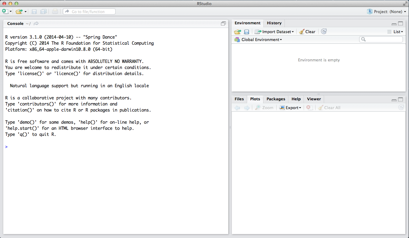
The panel in the upper right contains your workspace as well as a history of the commands that you’ve previously entered. Any plots that you generate will show up in the panel in the lower right corner.
The panel on the left is where the action happens. It’s called the console. Everytime you launch RStudio, it will have the same text at the top of the console telling you the version of R that you’re running. Below that information is the prompt. As its name suggests, this prompt is really a request, a request for a command. Initially, interacting with R is all about typing commands and interpreting the output. These commands and their syntax have evolved over decades (literally) and now provide what many users feel is a fairly natural way to access data and organize, describe, and invoke statistical computations.
Getting Started with R
Projects
In R, by default your files are saved to your working directory. To figure out where you working director is, you can use the following code:
getwd()
You can also tell R what folder to treat as your working directory. Go to Session -> Set Working Directory -> Choose Directory, then navigate to the folder location you would like to use.
Instead of constantly having to set or check your working directory, I strongly suggest working in an RStudio “Project” for this class.
RStudio projects are associated with R working directories. You can create an RStudio project in a brand new directory, in an existing directory (where you may already have code and data saved), or by cloning a git repository (advanced, and beyond the scope of this workshop).
When you create a Project, an .RProj file will be created in the directory. When you open a project, the working directory will automatically be set to the directory that the .RProj file is located in.
I also suggest creating a new Project for each research project you are working on. You can organize your folders and subfolders anyway you’d like. When you exit a project, you’ll be asked if you want to save your workspace. If you do choose to save, when you re-open the project at a later date, it will be as you last left it when you saved (everything in your history and environment preserved).
You can also have different projects open at one time, each in its own R Session.
For more information on Projects, see: https://support.rstudio.com/hc/en-us/articles/200526207-Using-Projects
RMD versus Script Files
R Scripts
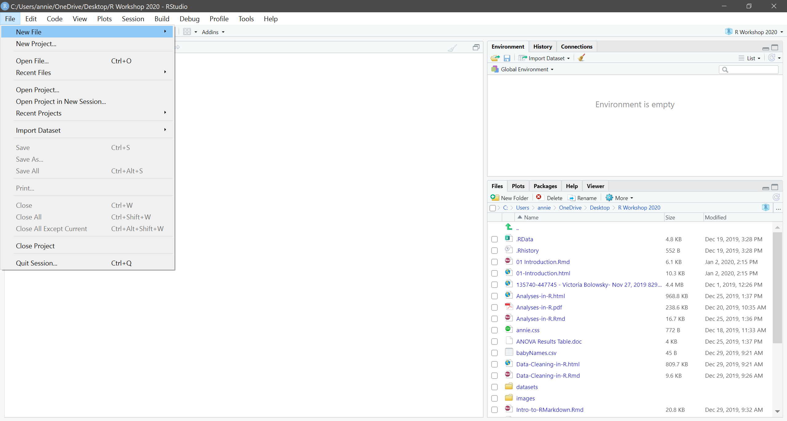
To open a new, clean script file, go to File -> New File -> R Script. Notice that it opens a new Pane in RStudio, and your Console area has now shifted down.You can also use the little button with the green plus sign under “File” to open a new file. If you like keyboard shortcuts, “Shift + CNTRL + N” will also open a new script file.
In a script file, you write you code and comments all in one place, but nothing actually runs until you send the code to the console. To send code to the console to run, highlight it and click the green “Run” button in the top right of the source pane. You can also put your cursor on the line of your code and then hit “CNTRL + ENTER” to get it to run.
- Type the following into your script file:
summary(cars)and then run the code (send it to the console).
RMD files
While script files are fine, we will be using RMarkdown (.Rmd) files this semester.
In an RMarkdown file, you can include text without having to comment it out.
Code for analyses is written in “Chunks” that can be run directly in the RMarkdown
document, with the output of the code chunk appearing right below. As you might
imagine, there are a lot of advantages to having your code, output, and text
describing or interpreting your analysis all in one place!
To open a new RMarkdown file, click on File -> New File -> RMarkdown… You will then be brought to the following screen:
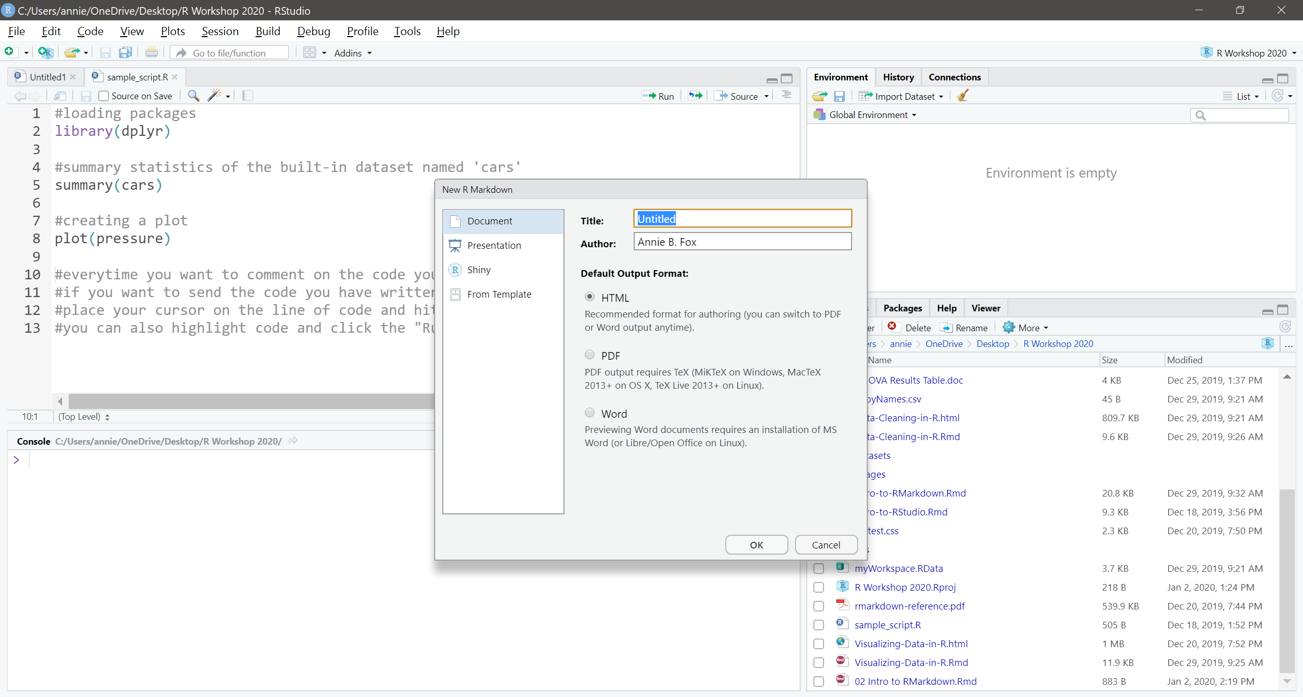
Give your document a title. Your name should automatically populate the “Author” field (you can change to whatever you want if you need to). Then click okay.
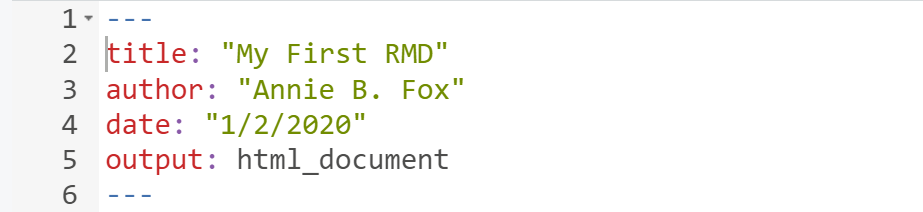
At the top of the new .Rmd file you just created, you’ll see what is called the “yaml” heading. This contains the title and author you provided on the previous screen, plus the date and output format. You can edit this as necessary. The information in the yaml is used when you “knit” the document (export to word, pdf, html, etc.).
Although we have created the document, we haven’t saved it. Click on the blue disk in the menu, and then save the rmd file to your workspace (give it whatever name you want).
Code Chunk Basics
When you open a new RMD file, sample code and text is provided. Note that there is both white space where text is present, and there are grey boxes where code is provided. These grey boxes are called “code chunks”. Code chunks are where you write your analyses. The white space before and after the code chunks can be used to take notes, write summaries, etc.
To create a new code chunk, you can click on the green “Insert” button in the top right menu, or you can use a keyboard shortcut (recommended):
Mac Users: On the last line in your new R Mardown file (or any blank line), click Command + Option + I
Windows Users: On the last line in your new R Markdown file (or any blank line), click Ctrl + Alt + I
You just created a new code chunk! It is within the code chunks themselves where you write code and load packages. Then, your code is sent to the Console to be evaluated/run.
#my first code chunk!
Chunk Titles
I find it helpful to give each of my code chunks a unique title. If you have a large RMD with many code chunks, it is helpful to label your code chunks with descriptive titles so you can navigate through your RMD quicker and more efficiently when you’re looking for something specific. This is a great way to keep your RMD organized. My advice would be that if you are running multiple tests to answer separate research questions, run each set of analyses in its own code chunk.
At the top of each chunk, you will see {r}. To name the code chunk, simply type in a name following the {r} with something like this: {r Factorial ANOVA}. You can name your code chunks whatever will be most helpful to you.
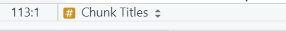
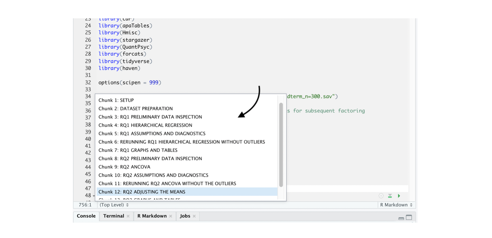
If you give your chunks names, you can navigate to those chunks using the “Chunk Titles” menu. You’ll find this menu at the bottom of your source pane and it looks like this:
When you click on “Chunk Titles” you will then see a list of all the chunks in the document. Here is an example:
Tips for Code Chunk Names
When naming your chunks, make sure NOT to:
Give multiple code chunks the same name. Make sure that each code chunk’s title is unique.
Alter the ``` at the top or bottom of your code chunk, nor the brackets { }. If you alter these, the code chunk no longer will function as such.
Use certain characters in the chunk titles. Generally, alphanumeric characters are acceptable within chunk titles, as are dashes. Including certain special characters in chunk titles can cause problems with some pacakges/when you’re trying to knit.
Running Code Chunks
There are two ways you can run code in a chunk. If you only want to run a specific section of your code, you can highlight the specific code that you want to run, like this:
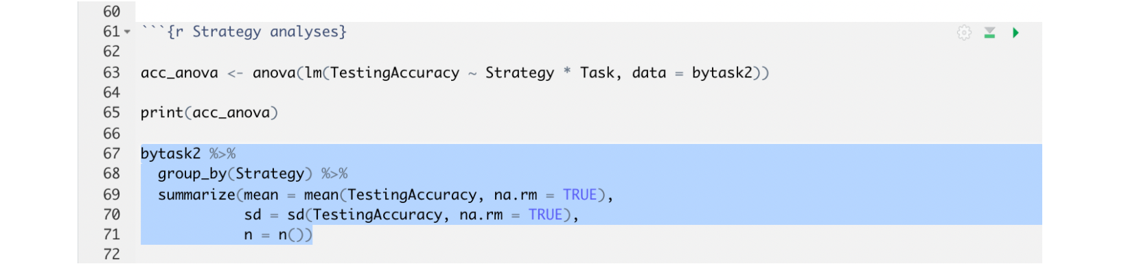
and then:
For Mac users, click Command + Return.
For Windows users, click Ctrl + Enter.
Alternatively, you can run it with your cursor at the very end of the code itself (i.e., after you’ve just typed in the last character). In the example below, the ‘very end’ is right after the n = ()). Your cursor can also be anywhere within that code itself, as illustrated below, and it will still run just that section, like this:
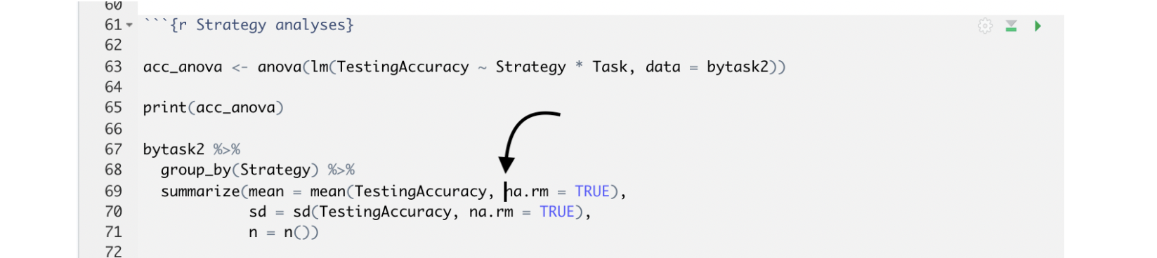
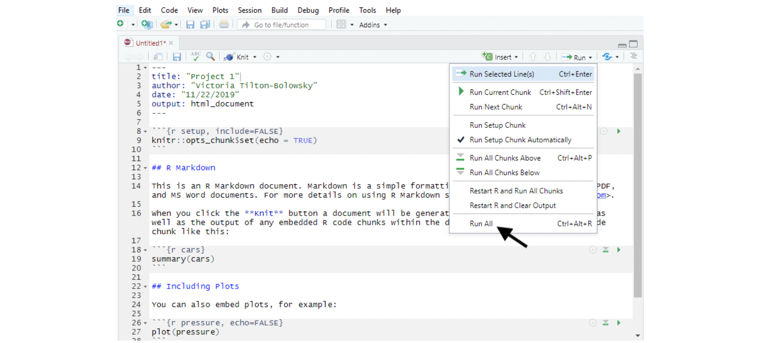
You can run an entire code chunk by clicking the right-pointing green arrow at the top right corner of the code chunk, or you can run your entire RMD file from top to bottom by clicking the Run All option shown here in this example.
Annotations within a Chunk
Here is another great way to organize your RMD and make your work clear to understand and remember - You can add annotations within your code chunks. You can do so by using the # character, and then typing your note. You can do this on a separate line from your code, or even on the same line as the code itself. Here is an example of annotating both ways within the same chunk. Just make sure you have the # symbol before your annotation, or else it will cause problems when you try to run the code chunk.
#Checking assumptions
leveneTest(EXAM ~ GENDER*FORMAT, data = class)

#Running a 2x2 factorial ANOVA
gendermod <- ezANOVA(data = class,
        dv = EXAM,
        between = .(GENDER, FORMAT), #the between-subjects independent variables
        wid = ID,
        type = 3,
        detailed = T,
        return_aov = T)

print(gendermod) #prints the results
Loading Data in R
There are several different methods you can use to use to get data into R that depend on the particular file type you are trying to import. R can read a wide variety of file types–text files, csv, spss, and so on. Some file types might require you to use specially designed packages to get the file into R.
Installing and using R packages
A large number of contributed packages are available for use in R. These packages are designed by R users to perform different types of tasks and analyses. If you are looking for a package for a specific task, https://cran.r-project.org/web/views/ and https://r-pkg.org are good places to start.
You can install a package in R using the install.packages() function. Once a
package is installed you have to “attach” (i.e., activate it) it in order to use
the functions it contains. To attach a package, use the library function.
You only need to install a package once, but you will need to attach it every
time you open a new session of R. The code below installs the package ‘readr’
which can be used to load datasets.
install.packages("readr")  ## installs the package
library(readr)  ##attaches the package
To make things a little easier going forward, we will install all of the packages we will need this semester now. Run the following code in your console:
install.packages(c("readr", "mosaic", "psych", "dplyr", "ggplot2", "tidyverse","MOTE", "apaTables", "car", "knitr", "kableExtra", "lsr", "DescTools","ez", "emmeans"))
Readers for common file types
In order to read data from a file, you have to know what kind of file it is. The table below lists functions that can import data from common plain-text formats.
| Data Type | Function |
|---|---|
| comma separated | read_csv() |
| tab separated | read_delim() |
| other delimited formats | read_table() |
| fixed width | read_fwf() |
You can also pull data from the Internet, which is what we will do here.
To get you started, run the following code. You can click the green arrow in the top right of the code chunk, or put your cursor at the end of the line of code and hit “CNTRL + ENTER” (or CMD + ENTER if you are on a mac).
source("http://www.openintro.org/stat/data/arbuthnot.R")
This command instructs R to access the OpenIntro website and fetch some data:
the Arbuthnot baptism counts for boys and girls. You should see that the
workspace area in the upper righthand corner of the RStudio window now lists a
data set called arbuthnot that has 82 observations on 3 variables. As you
interact with R, you will create a series of objects. Sometimes you load them as
we have done here, and sometimes you create them yourself as the byproduct of a
computation or some analysis you have performed. Note that because you are
accessing data from the web, this command (and the entire assignment) will work
anywhere you have access to the Internet.
Before we jump into looking at the data, let’s review some the basics for working in R.
R basics
Function calls
The general form for calling R functions is
## FunctionName(arg.1 = value.1, arg.2 = value.2, ..., arg.n - value.n)
Arguments can be matched by name; unnamed arguments will be matched by position.
Assignment
Values can be assigned names and used in subsequent operations
- The
<-operator (less than followed by a dash) is used to save values The name on the left gets the value on the right.
sqrt(10) ## calculate square root of 10; result is not stored anywhere
x <- sqrt(10) # assign result to a variable named x
Names should start with a letter, and contain only letters, numbers, underscores, and periods.
Data structures
There are two basic data structures in R: vectors and lists.
Vectors are of a particular type, e.g., integer, double, or character.
Vectors can be created using the c function, like this:
x <- c(1, 2, 3) # numeric vector
x
y <- c("a", "b", "c") # character vector
y
Lists are not restricted to a single type and can be used to hold
just about anything. They can be created using the list function,
like this:
z <- list(1, c(1, 2, 3, 4), list(c(1, 2), c("a", "b")))
z
The Data: Dr. Arbuthnot’s Baptism Records
The Arbuthnot data set refers to Dr. John Arbuthnot, an 18th century physician, writer, and mathematician. He was interested in the ratio of newborn boys to newborn girls, so he gathered the baptism records for children born in London for every year from 1629 to 1710. We can take a look at the data by typing its name into the console.
arbuthnot
What you should see are four columns of numbers, each row representing a different year: the first entry in each row is simply the row number (an index we can use to access the data from individual years if we want), the second is the year, and the third and fourth are the numbers of boys and girls baptized that year, respectively. Use the scrollbar on the right side of the console window to examine the complete data set.
Note that the row numbers in the first column are not part of Arbuthnot’s data. R adds them as part of its printout to help you make visual comparisons. You can think of them as the index that you see on the left side of a spreadsheet. In fact, the comparison to a spreadsheet will generally be helpful. R has stored Arbuthnot’s data in a kind of spreadsheet or table called a data frame.
You can see the dimensions of this data frame by typing:
dim(arbuthnot)
## [1] 82 3
This command should output [1] 82 3, indicating that there are 82 rows and 3
columns (we’ll get to what the [1] means in a bit), just as it says next to
the object in your workspace. You can see the names of these columns (or
variables) by typing:
names(arbuthnot)
## [1] "year" "boys" "girls"
You should see that the data frame contains the columns year, boys, and
girls. At this point, you might notice that many of the commands in R look a
lot like functions from math class; that is, invoking R commands means supplying
a function with some number of arguments. The dim and names commands, for
example, each took a single argument, the name of a data frame.
One advantage of RStudio is that it comes with a built-in data viewer. Click on
the name arbuthnot in the Environment pane (upper right window) that lists
the objects in your workspace. This will bring up an alternative display of the
data set in the Data Viewer (upper left window). You can close the data viewer
by clicking on the x in the upper lefthand corner.
Some Exploration
Let’s start to examine the data a little more closely. We can access the data in a single column of a data frame separately using a command like
arbuthnot$boys
This command will only show the number of boys baptized each year.
- What command would you use to extract just the counts of girls baptized? Try it!
Notice that the way R has printed these data is different. When we looked at the
complete data frame, we saw 82 rows, one on each line of the display. These data
are no longer structured in a table with other variables, so they are displayed
one right after another. Objects that print out in this way are called vectors;
they represent a set of numbers. R has added numbers in [brackets] along the
left side of the printout to indicate locations within the vector. For example,
5218 follows [1], indicating that 5218 is the first entry in the vector.
And if [43] starts a line, then that would mean the first number on that line
would represent the 43rd entry in the vector.
R has some powerful functions for making graphics. We can create a simple plot of the number of girls baptized per year with the command
plot(x = arbuthnot$year, y = arbuthnot$girls)
By default, R creates a scatterplot with each x,y pair indicated by an open
circle. The plot itself should appear under the Plots tab of the lower right
panel of RStudio. Notice that the command above again looks like a function,
this time with two arguments separated by a comma. The first argument in the
plot function specifies the variable for the x-axis and the second for the y-axis.
If we wanted to connect the data points with lines, we could add a third argument,
the letter l for line.
plot(x = arbuthnot$year, y = arbuthnot$girls, type = "l")
You might wonder how you are supposed to know that it was possible to add that third argument. Thankfully, R documents all of its functions extensively. To read what a function does and learn the arguments that are available to you, just type in a question mark followed by the name of the function that you’re interested in. Try the following.
?plot
Notice that the help file replaces the plot in the lower right panel. You can toggle between plots and help files using the tabs at the top of that panel.
- Is there an apparent trend in the number of girls baptized over the years?
How would you describe it?
Now, suppose we want to plot the total number of baptisms. To compute this, we could use the fact that R is really just a big calculator. We can type in mathematical expressions like
5218 + 4683
to see the total number of baptisms in 1629. We could repeat this once for each year, but there is a faster way. If we add the vector for baptisms for boys and girls, R will compute all sums simultaneously.
arbuthnot$boys + arbuthnot$girls
What you will see are 82 numbers (in that packed display, because we aren’t looking at a data frame here), each one representing the sum we’re after. Take a look at a few of them and verify that they are right. Therefore, we can make a plot of the total number of baptisms per year with the command
plot(arbuthnot$year, arbuthnot$boys + arbuthnot$girls, type = "l")
This time, note that we left out the names of the first two arguments. We can
do this because the help file shows that the default for plot is for the first
argument to be the x-variable and the second argument to be the y-variable.
Similarly to how we computed the proportion of boys, we can compute the ratio of the number of boys to the number of girls baptized in 1629 with
5218 / 4683
or we can act on the complete vectors with the expression
arbuthnot$boys / arbuthnot$girls
The proportion of newborns that are boys
5218 / (5218 + 4683)
or this may also be computed for all years simultaneously:
arbuthnot$boys / (arbuthnot$boys + arbuthnot$girls)
Note that with R as with your calculator, you need to be conscious of the order of operations. Here, we want to divide the number of boys by the total number of newborns, so we have to use parentheses. Without them, R will first do the division, then the addition, giving you something that is not a proportion.
- Now, make a plot of the proportion of boys over time. What do you see? Tip: If you use the up and down arrow keys, you can scroll through your previous commands, your so-called command history. You can also access it by clicking on the history tab in the upper right panel. This will save you a lot of typing in the future.
Finally, in addition to simple mathematical operators like subtraction and
division, you can ask R to make comparisons like greater than, >, less than,
<, and equality, ==. For example, we can ask if boys outnumber girls in each
year with the expression
arbuthnot$boys > arbuthnot$girls
This command returns 82 values of either TRUE if that year had more boys than
girls, or FALSE if that year did not (the answer may surprise you). This
output shows a different kind of data than we have considered so far. In the
arbuthnot data frame our values are numerical (the year, the number of boys
and girls). Here, we’ve asked R to create logical data, data where the values
are either TRUE or FALSE. In general, data analysis will involve many
different kinds of data types, and one reason for using R is that it is able to
represent and compute with many of them.
On Your Own
In the previous few pages, you recreated some of the displays and preliminary analysis of Arbuthnot’s baptism data. Your assignment involves repeating these steps, but for present day birth records in the United States. Load up the present day data with the following command.
source("http://www.openintro.org/stat/data/present.R")
The data are stored in a data frame called present.
What years are included in this data set? What are the dimensions of the data frame and what are the variable or column names?
How do these counts compare to Arbuthnot’s? Are they on a similar scale?
Make a plot that displays the boy-to-girl ratio for every year in the data set. What do you see? Does Arbuthnot’s observation about boys being born in greater proportion than girls hold up in the U.S.? Include the plot in your response.
In what year did we see the most total number of births in the U.S.?
You can refer to the help files or the R reference card http://cran.r-project.org/doc/contrib/Short-refcard.pdf to find helpful commands.
These data come from a report by the Centers for Disease Control http://www.cdc.gov/nchs/data/nvsr/nvsr53/nvsr53_20.pdf. Check it out if you would like to read more about an analysis of sex ratios at birth in the United States.
That was a short introduction to R and RStudio, but we will provide you with more functions and a more complete sense of the language as the course progresses. Feel free to browse around the websites for R and RStudio if you’re interested in learning more, or find more labs for practice at http://openintro.org.