Mixed Design ANOVA
We will use Field’s Looksorpersonality.sav data set for this exercise. This dataset is available on the website for the textbook here: DSUR Companion Website. You can also download a copy of the data here:Download Chick-Flick Dataset.
The “study” involved participants speed dating a set of potential dating partners and rating how much they would like to go on a real date with them at the end of the night. The attractiveness and personality of the dating partners was manipulated. Gender was also examined as a potential moderator. There are three independent variables—looks (attractive, average, ugly), personality (high charisma, some charisma, no charisma), and gender (male versus female).
Which IVs are within subjects? Which IVs are between subjects?
Write the null hypothesis(ses). Identify the dependent and independent variables and the types of data they represent.
Power Analysis for a Mixed Design ANOVA
Below are the inputs you’ll need to do a power analysis for a mixed design ANOVA using G*Power.
Test family: F-test
Statistical Test: Repeated measures, within-between interaction When conducting a mixed design ANOVA, often what the researcher is most interested in is the interaction between the independent variables. If you are only interested in the main effects, you would select the ANOVA for either repeated measures or between subjects (depending on which IV).
Estimate an effect size: Click “determine” and then “direct”.” Enter a partial eta square size you think might be accurate.
Alpha = .05
Power = .80
Number of groups = number of levels of between subjects
Number of measurements = number of levels of repeated measures
Corr among rep measures = correlation between levels or conditions. You’ll need pilot data or existing literature to select the appropriate sized correlation here, and you’ll want to use the lowest one you can find. If you aren’t sure, you can go with the default (.50), which is a reasonable correlation if you are measuring people multiple times. Use your judgement here, though. Higher correlations between repeated measures will require fewer participants.
Nonsphericity correction = epsilon This can be hard to estimate if you don’t have pilot data. If you do have pilot data, you can run a model and use the episilon value from that analysis. If not, leave it at the default.
Assumptions
In a mixed design ANOVA, you’ll need to deal with the assumptions of both a between subjects design and a repeated measures design.
Homogeneity of variance: You should take a look at the variances of each level of your between subjects independent variable. If the variances look different, you may have a problem. Remember that Levene’s Test is often significant with large sample sizes, so if you eye-balled the variances and they look okay, but Levene’s Test is significant, you’re probably fine to continue the analysis without having to worry.
One important thing to note is the ezANOVA doesn’t give Levene’s Test when you run a mixed design ANOVA. What you’ll need to do instead is run LeveneTest separately on just the between subjects IV.
Mauchly’s Test for Sphericity: With repeated measures data, we have to check the assumption of sphericity, which deals with whether the correlations between all of the levels of the repeated measures are equal (also known as compound symmetry). We need the variance of the difference scores between each combination of the levels of the repeated measures IV to be the same. Maulchy’s Test will be printed with the ezANOVA output. It is not uncommon to violate this assumption, and often people ignore it. If you do violate it, you can use either the GG or HF adjustments to the degrees of freedom, as we discussed previously.
The Looks or Personality Study
speed_dating <- read_sav("LooksOrPersonality.sav")
Let’s take a look a summary of the variables in the dataset.
summary(speed_dating)
##      Gender       att_high         av_high          ug_high
##  Min.   :1.0   Min.   : 80.00   Min.   : 69.00   Min.   :48.00
##  1st Qu.:1.0   1st Qu.: 85.50   1st Qu.: 82.50   1st Qu.:56.75
##  Median :1.5   Median : 89.00   Median : 86.50   Median :73.00
##  Mean   :1.5   Mean   : 88.95   Mean   : 85.60   Mean   :71.75
##  3rd Qu.:2.0   3rd Qu.: 92.00   3rd Qu.: 91.25   3rd Qu.:85.50
##  Max.   :2.0   Max.   :100.00   Max.   :100.00   Max.   :96.00
##     att_some        av_some         ug_some         att_none        av_none
##  Min.   :79.00   Min.   :59.00   Min.   :40.00   Min.   :45.00   Min.   :38.0
##  1st Qu.:83.00   1st Qu.:66.00   1st Qu.:46.75   1st Qu.:51.75   1st Qu.:46.5
##  Median :86.50   Median :71.00   Median :49.50   Median :68.00   Median :48.0
##  Mean   :87.80   Mean   :70.35   Mean   :49.75   Mean   :69.55   Mean   :47.4
##  3rd Qu.:92.75   3rd Qu.:74.00   3rd Qu.:53.25   3rd Qu.:86.25   3rd Qu.:50.0
##  Max.   :99.00   Max.   :79.00   Max.   :60.00   Max.   :97.00   Max.   :54.0
##     ug_none
##  Min.   :39.00
##  1st Qu.:45.00
##  Median :46.00
##  Mean   :45.95
##  3rd Qu.:47.00
##  Max.   :53.00
Cleaning, Screening, and Restructuring the Dataset
From the summary, we can see that we do not have an ID variable and we’ll need one to run ezANOVA. Our gender variable also needs to be factored. Also note that each column represents information from two different repeated measures variables. We will need to restructure the data and separate the IVs. Like we did with repeated measures ANOVAs, we will use gather and separate from tidyr to restructure the data.
Below, I use the %>% to do all of these steps in one code chunk. First, the ID variable is created.Then the data is restructured, and then the gender and newly created variables are factored. Note that for the gender variable, 1=male and 2=female.
men <-speed_dating %>%
  subset(Gender=="1")
women <- speed_dating %>%
  subset(Gender=="2")

men %>%
  select(att_high:ug_none) %>%    #selecting only the 4 repeated measures variables
  cor(use = "pairwise.complete.obs")
##              att_high     av_high      ug_high    att_some    av_some
## att_high  1.000000000  0.32465212  0.002041894 -0.32790587  0.3956216
## av_high   0.324652117  1.00000000 -0.037088396  0.02210869 -0.2707663
## ug_high   0.002041894 -0.03708840  1.000000000 -0.64178422  0.3362128
## att_some -0.327905866  0.02210869 -0.641784224  1.00000000 -0.5697296
## av_some   0.395621582 -0.27076627  0.336212843 -0.56972955  1.0000000
## ug_some   0.392183880  0.22306790  0.009376720 -0.03420906 -0.1703213
## att_none -0.257893665  0.28763382  0.347996732  0.05518193 -0.3164255
## av_none   0.189226584  0.58602595  0.229800704 -0.43484792  0.1238303
## ug_none   0.226385515 -0.40453187 -0.148224308  0.19445147  0.2919794
##              ug_some    att_none    av_none    ug_none
## att_high  0.39218388 -0.25789367  0.1892266  0.2263855
## av_high   0.22306790  0.28763382  0.5860260 -0.4045319
## ug_high   0.00937672  0.34799673  0.2298007 -0.1482243
## att_some -0.03420906  0.05518193 -0.4348479  0.1944515
## av_some  -0.17032130 -0.31642545  0.1238303  0.2919794
## ug_some   1.00000000 -0.45955097 -0.2933852 -0.2560554
## att_none -0.45955097  1.00000000  0.2422039 -0.0821034
## av_none  -0.29338517  0.24220390  1.0000000 -0.0103722
## ug_none  -0.25605536 -0.08210340 -0.0103722  1.0000000
women %>%
  select(att_high:ug_none) %>%    #selecting only the 4 repeated measures variables
  cor(use = "pairwise.complete.obs")
##              att_high     av_high     ug_high    att_some     av_some
## att_high  1.000000000  0.08361709  0.62134370  0.06248143  0.47138953
## av_high   0.083617092  1.00000000  0.36112198 -0.44570044  0.17121218
## ug_high   0.621343704  0.36112198  1.00000000 -0.03212517 -0.05938769
## att_some  0.062481428 -0.44570044 -0.03212517  1.00000000 -0.19170523
## av_some   0.471389530  0.17121218 -0.05938769 -0.19170523  1.00000000
## ug_some  -0.003684439  0.14727261  0.12591393  0.52633211  0.23688403
## att_none -0.095872098  0.49305262 -0.02718500 -0.23985105 -0.04966546
## av_none   0.143185118 -0.12834702 -0.33313643  0.46685558  0.12970622
## ug_none   0.154809523  0.16330615  0.45440638 -0.08557681  0.17685278
##               ug_some    att_none     av_none     ug_none
## att_high -0.003684439 -0.09587210  0.14318512  0.15480952
## av_high   0.147272612  0.49305262 -0.12834702  0.16330615
## ug_high   0.125913932 -0.02718500 -0.33313643  0.45440638
## att_some  0.526332113 -0.23985105  0.46685558 -0.08557681
## av_some   0.236884029 -0.04966546  0.12970622  0.17685278
## ug_some   1.000000000 -0.25105011  0.11436443  0.05838291
## att_none -0.251050106  1.00000000  0.30059146  0.37874647
## av_none   0.114364429  0.30059146  1.00000000 -0.01933708
## ug_none   0.058382915  0.37874647 -0.01933708  1.00000000
speed_long <- speed_dating %>%
  mutate(id = row_number()) %>%
  gather(key = "key", value = "Rating", att_high:ug_none) %>%
  arrange(id) %>%
  separate(key, into = c("Looks", "Personality"), sep = "_") %>%
  mutate(Looks = factor(Looks,
                        levels = c("att", "av", "ug"),
                        labels = c("Attractive", "Average", "Ugly")),
         Personality = factor(Personality,
                          levels = c("high", "some", "none"),
                          labels = c("Charismatic", "Average", "Dullard")),
         Gender = factor(Gender,
                         levels = c(1,2),
                         labels = c("Male", "Female")))
## Warning: attributes are not identical across measure variables;
## they will be dropped
summary(speed_long)
##     Gender         id               Looks         Personality     Rating
##  Male  :90   Min.   : 1.00   Attractive:60   Charismatic:60   Min.   : 38.00
##  Female:90   1st Qu.: 5.75   Average   :60   Average    :60   1st Qu.: 50.00
##              Median :10.50   Ugly      :60   Dullard    :60   Median : 70.00
##              Mean   :10.50                                    Mean   : 68.57
##              3rd Qu.:15.25                                    3rd Qu.: 86.00
##              Max.   :20.00                                    Max.   :100.00
Now we will take a look at the descriptive statistics as a function of all three of our independent variables.
favstats(Rating ~ Gender+Looks+Personality, data = speed_long)
##         Gender.Looks.Personality min    Q1 median    Q3 max mean       sd  n
## 1    Male.Attractive.Charismatic  80 86.75   89.0 89.75 100 88.3 5.696978 10
## 2  Female.Attractive.Charismatic  80 84.50   89.0 95.00  99 89.6 6.636599 10
## 3       Male.Average.Charismatic  69 81.50   84.0 85.75  94 82.8 7.004760 10
## 4     Female.Average.Charismatic  69 87.50   90.5 92.00 100 88.4 8.329332 10
## 5          Male.Ugly.Charismatic  48 53.25   56.5 60.25  67 56.8 5.731007 10
## 6        Female.Ugly.Charismatic  79 83.50   86.0 89.75  96 86.7 5.437524 10
## 7        Male.Attractive.Average  80 86.00   87.5 91.00  99 88.5 5.739725 10
## 8      Female.Attractive.Average  79 81.50   86.0 93.25  98 87.1 6.806043 10
## 9           Male.Average.Average  63 70.25   71.0 73.75  79 71.8 4.417138 10
## 10        Female.Average.Average  59 65.25   68.0 73.50  79 68.9 5.952590 10
## 11             Male.Ugly.Average  40 45.00   48.5 50.00  58 48.3 5.375872 10
## 12           Female.Ugly.Average  43 47.00   52.0 53.75  60 51.2 5.452828 10
## 13       Male.Attractive.Dullard  78 84.50   86.5 90.75  97 87.3 5.437524 10
## 14     Female.Attractive.Dullard  45 50.25   51.5 53.50  58 51.8 3.457681 10
## 15          Male.Average.Dullard  38 47.25   48.0 50.00  54 47.8 4.184628 10
## 16        Female.Average.Dullard  39 45.50   48.0 48.00  53 47.0 3.741657 10
## 17             Male.Ugly.Dullard  39 45.00   45.5 47.00  53 45.8 3.583915 10
## 18           Female.Ugly.Dullard  40 45.00   46.5 47.00  52 46.1 3.071373 10
##    missing
## 1        0
## 2        0
## 3        0
## 4        0
## 5        0
## 6        0
## 7        0
## 8        0
## 9        0
## 10       0
## 11       0
## 12       0
## 13       0
## 14       0
## 15       0
## 16       0
## 17       0
## 18       0
Levene’s Test
leveneTest(Rating~Gender, data=speed_long)
## Levene's Test for Homogeneity of Variance (center = median)
##        Df F value Pr(>F)
## group   1  0.7678 0.3821
##       178
Running the ANOVA
We will use ezANOVA to run the ANOVA model. We have one between subjects variable, Gender, and two within subjects variables, Looks and Personality. Request Type 3 Sums of Squares, as well as return_aov = TRUE. We will need the aov results to run post-hoc comparisons later (if any of our interactions are significant).
options(digits = 3)
options(scipen =999)
options(contrasts = c("contr.sum", "contr.poly"))
speedModel<-ezANOVA(data = speed_long,
                    dv = .(Rating),
                    wid = .(id),
                    between = .(Gender),
                    within = .(Looks, Personality),
                    type = 3,
                    detailed = TRUE,
                    return_aov = TRUE)
## Warning: Converting "id" to factor for ANOVA.
print(speedModel)
## $ANOVA
##                     Effect DFn DFd      SSn  SSd           F
## 1              (Intercept)   1  18 846249.8  760 20036.89968
## 2                   Gender   1  18      0.2  760     0.00474
## 3                    Looks   2  36  20779.6  883   423.73252
## 5              Personality   2  36  23233.6 1274   328.24977
## 4             Gender:Looks   2  36   3944.1  883    80.42699
## 6       Gender:Personality   2  36   4420.1 1274    62.44868
## 7        Looks:Personality   4  72   4055.3 1993    36.63253
## 8 Gender:Looks:Personality   4  72   2669.7 1993    24.11596
##                                   p p<.05       ges
## 1 0.0000000000000000000000000000701     * 0.9942319
## 2 0.9458958475568546298006822325988       0.0000407
## 3 0.0000000000000000000000000959481     * 0.8088849
## 5 0.0000000000000000000000076894298     * 0.8255493
## 4 0.0000000000000523418671863051214     * 0.4454748
## 6 0.0000000000019749859639075176266     * 0.4737685
## 7 0.0000000000000001101308132536972     * 0.4523510
## 8 0.0000000000011078009545646184235     * 0.3522328
##
## $`Mauchly's Test for Sphericity`
##                     Effect     W     p p<.05
## 3                    Looks 0.960 0.708
## 4             Gender:Looks 0.960 0.708
## 5              Personality 0.929 0.536
## 6       Gender:Personality 0.929 0.536
## 7        Looks:Personality 0.613 0.534
## 8 Gender:Looks:Personality 0.613 0.534
##
## $`Sphericity Corrections`
##                     Effect   GGe                         p[GG] p[GG]<.05   HFe
## 3                    Looks 0.962 0.000000000000000000000000762         * 1.074
## 4             Gender:Looks 0.962 0.000000000000148702643589779         * 1.074
## 5              Personality 0.934 0.000000000000000000000205662         * 1.038
## 6       Gender:Personality 0.934 0.000000000009442425658493532         * 1.038
## 7        Looks:Personality 0.799 0.000000000000090035984243933         * 0.992
## 8 Gender:Looks:Personality 0.799 0.000000000147042182668051506         * 0.992
##                            p[HF] p[HF]<.05
## 3 0.0000000000000000000000000959         *
## 4 0.0000000000000523418671863051         *
## 5 0.0000000000000000000000076894         *
## 6 0.0000000000019749859639075176         *
## 7 0.0000000000000001426883124759         *
## 8 0.0000000000013378764445001671         *
##
## $aov
##
## Call:
## aov(formula = formula(aov_formula), data = data)
##
## Grand Mean: 68.6
##
## Stratum 1: id
##
## Terms:
##                 Gender Residuals
## Sum of Squares       0       760
## Deg. of Freedom      1        18
##
## Residual standard error: 6.5
## Estimated effects are balanced
##
## Stratum 2: id:Looks
##
## Terms:
##                 Looks Gender:Looks Residuals
## Sum of Squares  20780         3944       883
## Deg. of Freedom     2            2        36
##
## Residual standard error: 4.95
## Estimated effects may be unbalanced
##
## Stratum 3: id:Personality
##
## Terms:
##                 Personality Gender:Personality Residuals
## Sum of Squares        23234               4420      1274
## Deg. of Freedom           2                  2        36
##
## Residual standard error: 5.95
## Estimated effects may be unbalanced
##
## Stratum 4: id:Looks:Personality
##
## Terms:
##                 Looks:Personality Gender:Looks:Personality Residuals
## Sum of Squares               4055                     2670      1993
## Deg. of Freedom                 4                        4        72
##
## Residual standard error: 5.26
## Estimated effects may be unbalanced
Based on the results of the ANOVA, there is a main effect of Looks and a main effect of Personality. The main effect of gender is not statistically significant. All of the interactions are statistically significant. In the presence of significant interactions, we could bypass looking at the main effects. But for practice, let’s go ahead and graph the means for each main effect, as well as look at post-hoc comparisons to see which groups are different from one another.
Examining the Main Effects
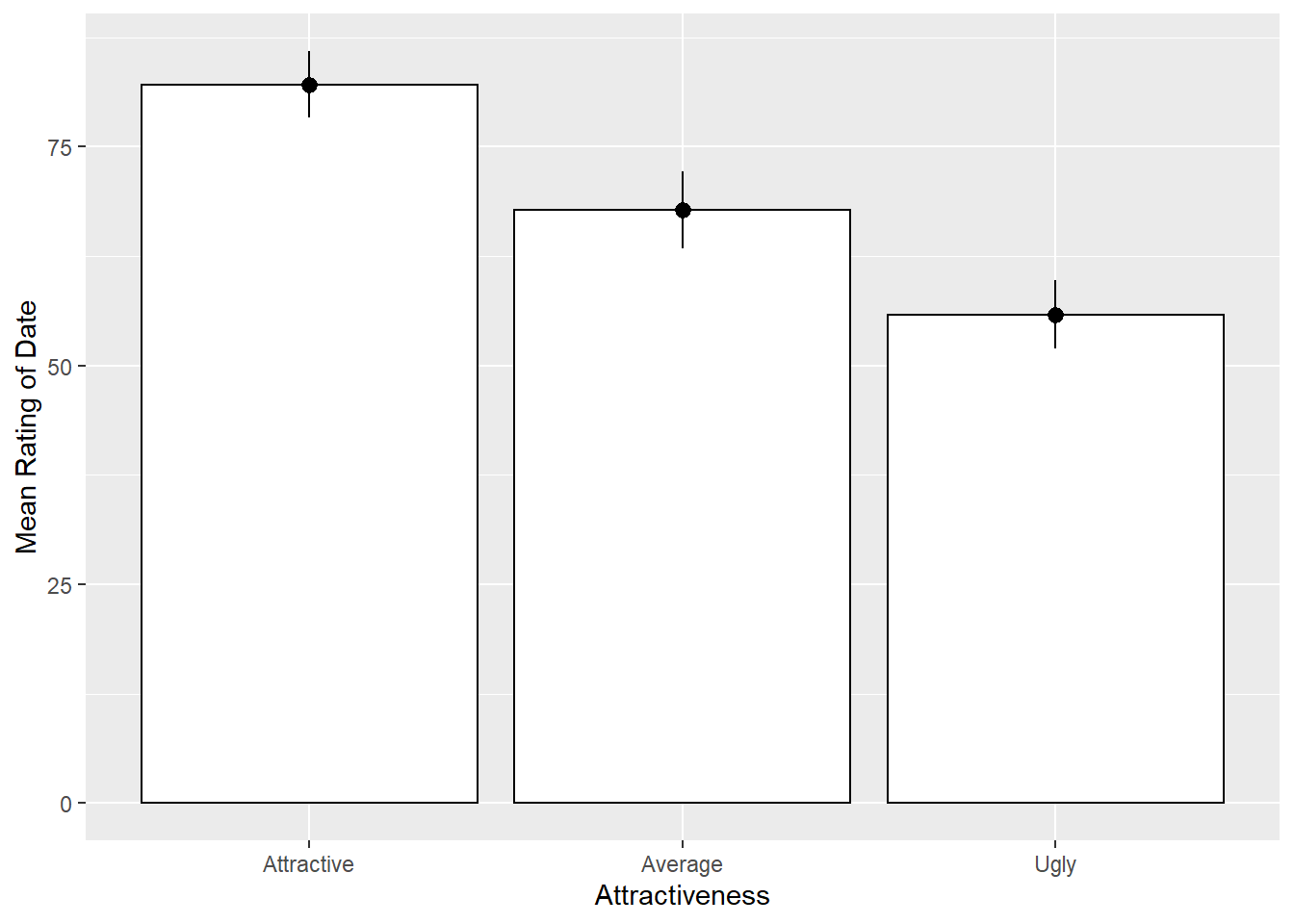
#Bar Graph for Looks
looksBar <- ggplot(speed_long, aes(Looks, Rating))
looksBar + stat_summary(fun.y = mean,
                        geom = "bar",
                        fill = "White",
                        colour = "Black") +
  stat_summary(fun.data = mean_cl_normal, geom = "pointrange") +
  labs(x = "Attractiveness", y = "Mean Rating of Date")
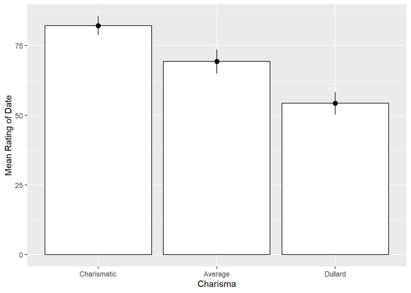
#Bar Graph for Personality
personalityBar <- ggplot(speed_long, aes(Personality, Rating))
personalityBar + stat_summary(fun.y = mean,
                        geom = "bar",
                        fill = "White",
                        colour = "Black") +
  stat_summary(fun.data = mean_cl_normal, geom = "pointrange") +
  labs(x = "Charisma", y = "Mean Rating of Date")
pairwise.t.test(speed_long$Rating, speed_long$Looks,
                paired = T,
                var.equal = T,
                p.adjust.method = "bonferroni")
##
## 	Pairwise comparisons using paired t tests
##
## data:  speed_long$Rating and speed_long$Looks
##
##         Attractive           Average
## Average 0.000000002          -
## Ugly    < 0.0000000000000002 0.000000003
##
## P value adjustment method: bonferroni
pairwise.t.test(speed_long$Rating, speed_long$Personality,
                paired = T,
                var.equal = T,
                p.adjust.method = "bonferroni")
##
## 	Pairwise comparisons using paired t tests
##
## data:  speed_long$Rating and speed_long$Personality
##
##         Charismatic          Average
## Average 0.0000000206         -
## Dullard < 0.0000000000000002 0.0000000002
##
## P value adjustment method: bonferroni
For both of the main effects, all three conditions are significantly different than one another.
Interactions
There are three significant two-way interactions and a significant three way interaction. We should just focus on the significant 3-way interaction and ignore the two-way interactions. But let’s take a look at one of the two-way interactions just for practice.
Gender x Looks Interaction
There are two ways we could look at the gender x looks interaction: We could break it down by looking at the effect of gender at each level of Looks, or, we could look at the effect of looks separately for men and women. How do you decide which way to do it?
1.) What are your hypotheses? Break down the interaction in a way that makes the most sense for the question(s) you are trying to answer.
2.) Break it down in the way that requires the fewest number of tests. This will protect your Type I error rate.
For this exercise, we will look at the effect of gender at each level of Looks. One important thing to pay attention to when doing the post-hocs for a mixed ANOVA is whether the test you are doing is between subjects or within subjects. Because Gender is our between subjects variable and we will be comparing men and women at each level of Looks, we should use independent samples t-tests. (If we broke the interaction down the other way, we would need to use dependent samples t-tests).
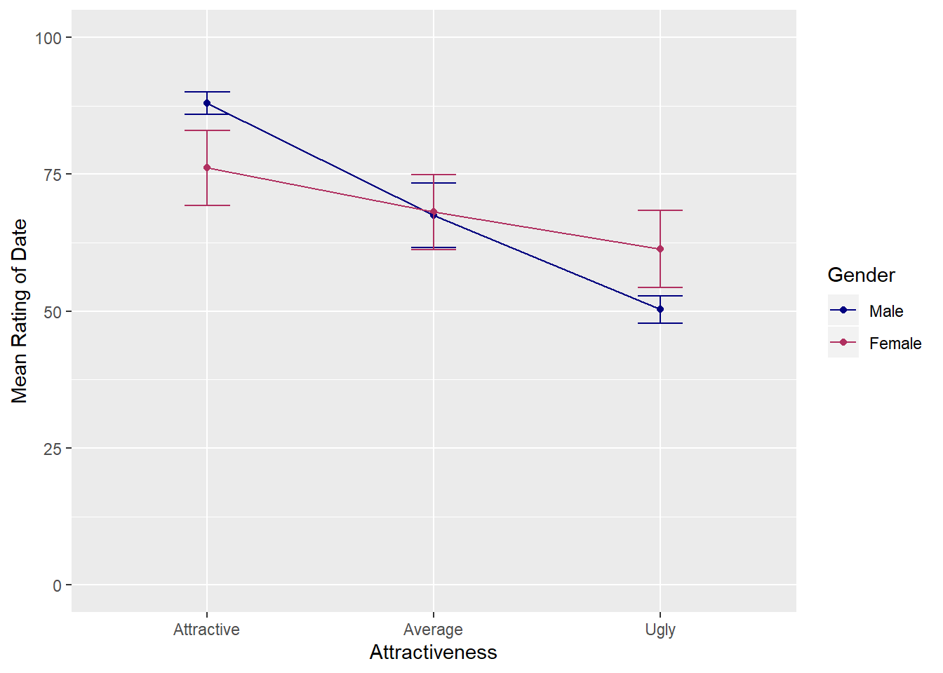
Before we conduct the simple effects analyses, let’s plot the 2-way interaction between gender and looks.
#Plot of the interaction
genderLooks <- ggplot(speed_long, aes(Looks, Rating, colour = Gender))
genderLooks +
  stat_summary(fun.y = mean, geom = "point") +
  stat_summary(fun.y = mean, geom = "line", aes(group= Gender)) +
  stat_summary(fun.data = mean_cl_normal, geom = "errorbar", width = 0.2) +
  labs(x = "Attractiveness", y = "Mean Rating of Date", colour = "Gender") +
  scale_y_continuous(limits = c(0,100)) +
  scale_colour_manual(values= c("navy", "maroon"))
speed_long %>%
  dplyr::filter(Looks=="Attractive") %>%
  t.test(Rating~Gender, data=., var.equal=TRUE)
##
## 	Two Sample t-test
##
## data:  Rating by Gender
## t = 3, df = 58, p-value = 0.001
## alternative hypothesis: true difference in means is not equal to 0
## 95 percent confidence interval:
##   4.84 18.89
## sample estimates:
##   mean in group Male mean in group Female
##                 88.0                 76.2
speed_long %>%
  dplyr::filter(Looks=="Average") %>%
  t.test(Rating~Gender, data=., var.equal=TRUE)
##
## 	Two Sample t-test
##
## data:  Rating by Gender
## t = -0.1, df = 58, p-value = 0.9
## alternative hypothesis: true difference in means is not equal to 0
## 95 percent confidence interval:
##  -9.44  8.17
## sample estimates:
##   mean in group Male mean in group Female
##                 67.5                 68.1
speed_long %>%
  dplyr::filter(Looks=="Ugly") %>%
  t.test(Rating~Gender, data=., var.equal=TRUE)
##
## 	Two Sample t-test
##
## data:  Rating by Gender
## t = -3, df = 58, p-value = 0.004
## alternative hypothesis: true difference in means is not equal to 0
## 95 percent confidence interval:
##  -18.39  -3.68
## sample estimates:
##   mean in group Male mean in group Female
##                 50.3                 61.3
From the results of the post-hoc tests and an examination of the graph, we can see that for attractive dates, men rated the date higher than women. When the date was ugly, women rated the date higher than men. At an average level of atttractiveness, there was no difference in ratings between men and women.
Using emmeans to conduct post-hoc tests and contrasts
The emmeans package can be used to conduct contrasts and pairwise comparisons. It will also give you the marginal means and standard errors as a function of your independent variables.
#marginal means by IVs with contrasts
genderlooks_emm <- emmeans(speedModel$aov, pairwise ~ Gender|Looks)
## NOTE: Results may be misleading due to involvement in interactions
genderlooks_emm
## $emmeans
## Looks = Attractive:
##  Gender emmean   SE   df lower.CL upper.CL
##  Male     88.0 1.01 50.2     86.0     90.1
##  Female   76.2 1.01 50.2     74.1     78.2
##
## Looks = Average:
##  Gender emmean   SE   df lower.CL upper.CL
##  Male     67.5 1.01 50.2     65.4     69.5
##  Female   68.1 1.01 50.2     66.1     70.1
##
## Looks = Ugly:
##  Gender emmean   SE   df lower.CL upper.CL
##  Male     50.3 1.01 50.2     48.3     52.3
##  Female   61.3 1.01 50.2     59.3     63.4
##
## Results are averaged over the levels of: Personality
## Warning: EMMs are biased unless design is perfectly balanced
## Confidence level used: 0.95
##
## $contrasts
## Looks = Attractive:
##  contrast      estimate   SE   df t.ratio p.value
##  Male - Female    11.87 1.42 50.2  8.330  <.0001
##
## Looks = Average:
##  contrast      estimate   SE   df t.ratio p.value
##  Male - Female    -0.63 1.42 50.2 -0.440  0.6580
##
## Looks = Ugly:
##  contrast      estimate   SE   df t.ratio p.value
##  Male - Female   -11.03 1.42 50.2 -7.750  <.0001
##
## Results are averaged over the levels of: Personality
- Analyze and interpret the other significant two-way interactions. Include a plot of the means.
Three-way Interaction
Gender x Looks x Personality Interaction
Here is where things get a bit more complicated. We have a significant three way interaction. What that means is that the interaction between Looks and Personality depends on whether you are male or female. Before we break down the interaction for significance testing, let’s graph it first. To graph a three-way interaction, we will want to use facet_wrap so that we get separate plots of Looks x Personality for men and women. This wil allow us to visualize the interaction separately for men and women.
looksCharismaGender <- ggplot(speed_long, aes(Looks, Rating, colour = Personality))
looksCharismaGender +
  stat_summary(fun.y = mean, geom = "point") +
  stat_summary(fun.y = mean, geom = "line", aes(group= Personality)) +
  stat_summary(fun.data = mean_cl_boot, geom = "errorbar", width = 0.2) +
  labs(x = "Attractiveness", y = "Mean Rating of Date", colour = "Charisma") +
  scale_y_continuous(limits = c(0,100)) +
  facet_wrap(~Gender)
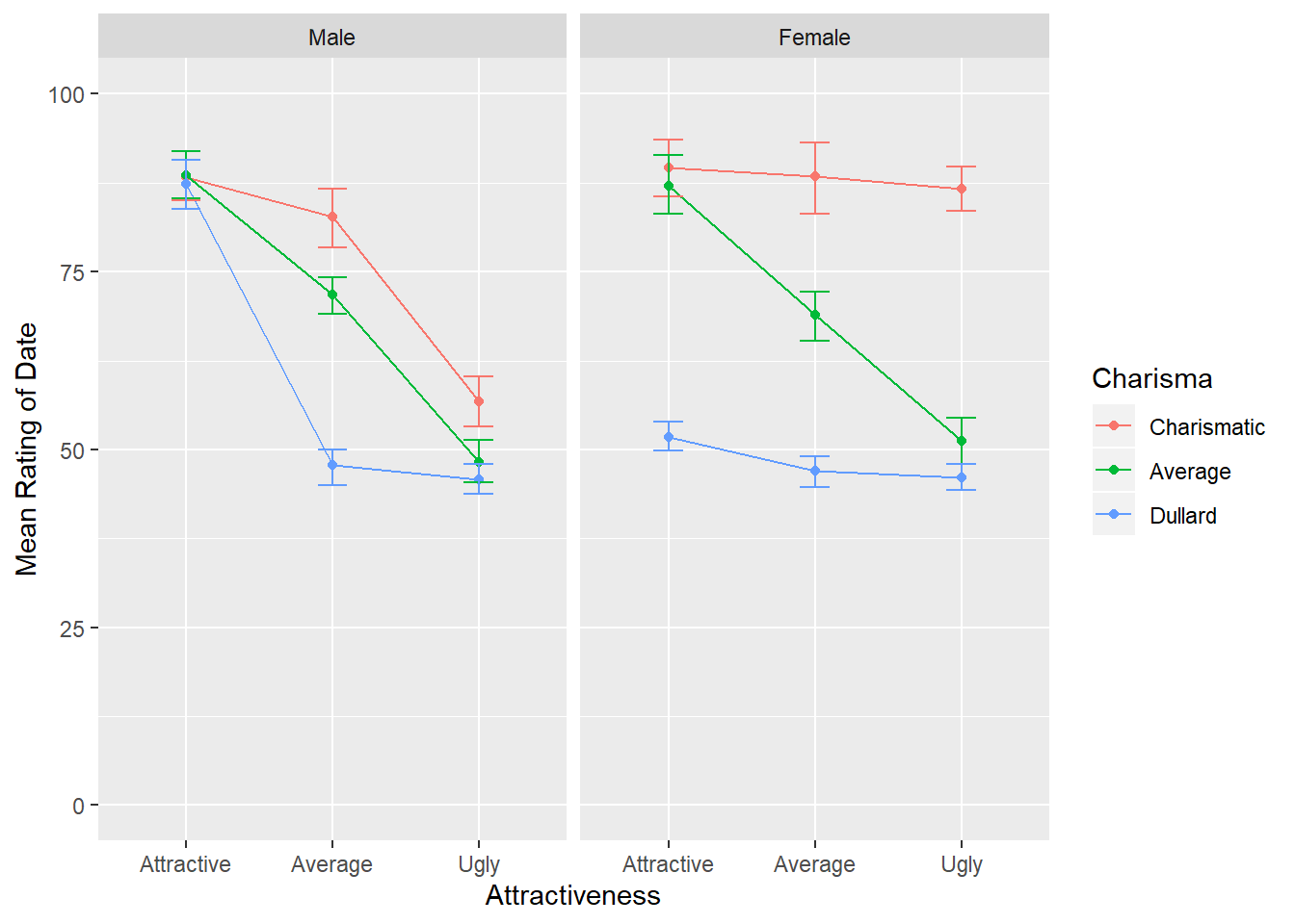 From the graph, we can see that the interaction betwen Looks and Personality is different for men and women. For men, for the Attractive date and the Ugly date, there doesn’t appear to be any major differences in the ratings based on personality. But for average attractiveness, the mean ratings of the date vary by their level of personality. Further, it looks like there is a general negative trend between attractiveness and personality. As attractiveness and charisma decrease, ratings of the date decreased.
For women, attractiveness seems to have the largest effect for those who were average in charisma. For average personalities, mean ratings of the date decrease as attractiveness decreases. Attractiveness does not seem to affect ratings for the charismatic or dullard personalities (although we can see that the charismatic ratings are higher across the board than those for the dullard). Now let’s do the simple effects analysis.
We’ll use the emmeans function to do this set of simple effects analyses. First, we’ll take a look at the marginal means as a function of all three independent variables. Then will use contrast to look at a contrast of the contrasts.
emm_threeway <- emmeans(speedModel$aov, ~Personality*Looks*Gender)
emm_threeway
##  Personality Looks      Gender emmean   SE  df lower.CL upper.CL
##  Charismatic Attractive Male     88.3 1.74 156     84.9     91.7
##  Average     Attractive Male     88.5 1.74 156     85.1     91.9
##  Dullard     Attractive Male     87.3 1.74 156     83.9     90.7
##  Charismatic Average    Male     82.8 1.74 156     79.4     86.2
##  Average     Average    Male     71.8 1.74 156     68.4     75.2
##  Dullard     Average    Male     47.8 1.74 156     44.4     51.2
##  Charismatic Ugly       Male     56.8 1.74 156     53.4     60.2
##  Average     Ugly       Male     48.3 1.74 156     44.9     51.7
##  Dullard     Ugly       Male     45.8 1.74 156     42.4     49.2
##  Charismatic Attractive Female   89.6 1.74 156     86.2     93.0
##  Average     Attractive Female   87.1 1.74 156     83.7     90.5
##  Dullard     Attractive Female   51.8 1.74 156     48.4     55.2
##  Charismatic Average    Female   88.4 1.74 156     85.0     91.8
##  Average     Average    Female   68.9 1.74 156     65.5     72.3
##  Dullard     Average    Female   47.0 1.74 156     43.6     50.4
##  Charismatic Ugly       Female   86.7 1.74 156     83.3     90.1
##  Average     Ugly       Female   51.2 1.74 156     47.8     54.6
##  Dullard     Ugly       Female   46.1 1.74 156     42.7     49.5
##
## Warning: EMMs are biased unless design is perfectly balanced
## Confidence level used: 0.95
emm_comparisons <- contrast(emm_threeway, interaction = c("consec", "consec", "consec"))
emm_comparisons
##  Personality_consec    Looks_consec         Gender_consec estimate   SE df
##  Average - Charismatic Average - Attractive Female - Male     -5.8 4.71 72
##  Dullard - Average     Average - Attractive Female - Male     36.2 4.71 72
##  Average - Charismatic Ugly - Average       Female - Male    -18.5 4.71 72
##  Dullard - Average     Ugly - Average       Female - Male     -4.7 4.71 72
##  t.ratio p.value
##  -1.230  0.2220
##   7.690  <.0001
##  -3.930  <.0001
##  -1.000  0.3210
How do we interpret these results? The first contrast “Average-Charismatic” “Average-Attractive” “Female-Male” looks at whether the difference between average and charismatic ratings at average and attractive looks differ for men and women. Confused? Plots of each of the contrasts should help us understand what these comparisons are telling us.
contrast1 <- speed_long %>%
  dplyr::filter(Personality=="Average" | Personality == "Charismatic") %>%
  dplyr::filter(Looks == "Average" | Looks == "Attractive") %>%
  ggplot(aes(Looks, Rating, color=Personality)) +
    stat_summary(fun.y = mean, geom = "point") +
    stat_summary(fun.y = mean, geom = "line", aes(group= Personality)) +
    stat_summary(fun.data = mean_cl_boot, geom = "errorbar", width = 0.2) +
    labs(x = "Attractiveness", y = "Mean Rating of Date", colour = "Charisma") +
    scale_y_continuous(limits = c(0,100)) +
    scale_color_manual(values = c("#F8766D", "#00BA38")) +
    facet_wrap(~Gender) +
    ggtitle("Contrast 1: Average v Charismatic, Attractive v Average, Men v Women")
contrast1
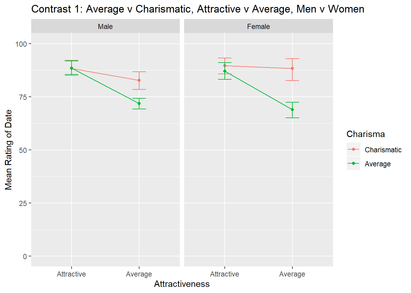
What we are calling contrast 1 here compares ratings of attractive versus average when high charisma is compared to average charisma in men compared to women. We can see in the graph that for both men and women, the attractive date was rated similarly whether the date had a high or average level of charisma. Ratings for the average looking date, ratings of the date were higher when charisma was high compared to average. The pattern of results is similar for men and women, which is why the contrast for this part of the interaction is not statistically significant.
contrast2 <- speed_long %>%
  dplyr::filter(Personality=="Average" | Personality == "Dullard") %>%
  dplyr::filter(Looks == "Average" | Looks == "Attractive") %>%
  ggplot(aes(Looks, Rating, color=Personality)) +
    stat_summary(fun.y = mean, geom = "point") +
    stat_summary(fun.y = mean, geom = "line", aes(group= Personality)) +
    stat_summary(fun.data = mean_cl_boot, geom = "errorbar", width = 0.2) +
    labs(x = "Attractiveness", y = "Mean Rating of Date", colour = "Charisma") +
    scale_y_continuous(limits = c(0,100)) +
    scale_color_manual(values=c("#619CFF","#00BA38")) +
    facet_wrap(~Gender) +
    ggtitle("Contrast 2: Average v Dullard, Attractive v Average, Men v Women")
contrast2
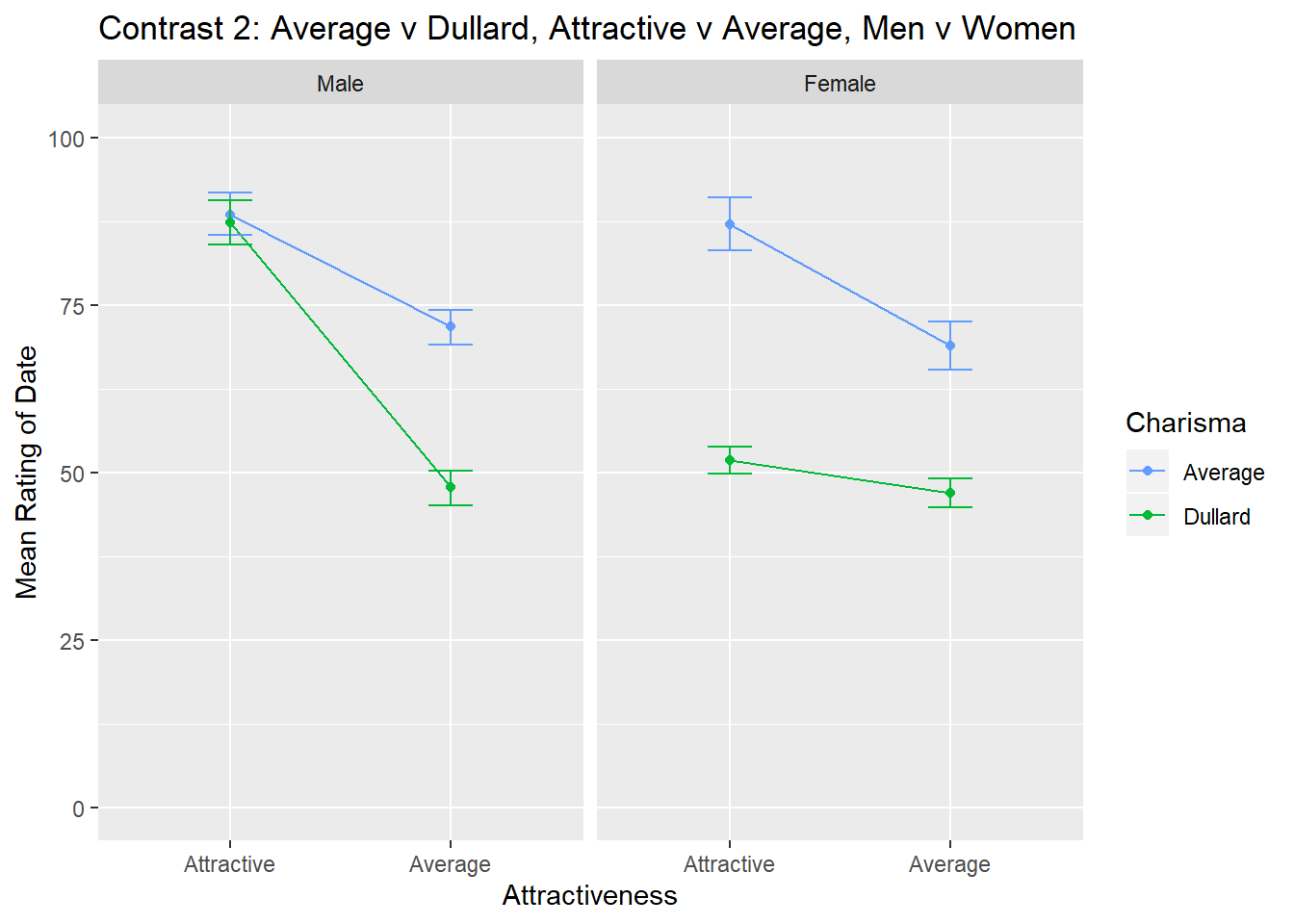
Constrast 2 compares attractive versus average Looks for average versus dullard personalities for men and women. Here we can see that the pattern of results is different for men and women.
contrast3 <- speed_long %>%
  filter(Personality=="Average" | Personality == "Charismatic") %>%
  filter(Looks == "Average" | Looks == "Ugly") %>%
  ggplot(aes(Looks, Rating, color=Personality)) +
    stat_summary(fun.y = mean, geom = "point") +
    stat_summary(fun.y = mean, geom = "line", aes(group= Personality)) +
    stat_summary(fun.data = mean_cl_boot, geom = "errorbar", width = 0.2) +
    labs(x = "Attractiveness", y = "Mean Rating of Date", colour = "Charisma") +
    scale_y_continuous(limits = c(0,100)) +
    scale_color_manual(values= c("#F8766D", "#00BA38")) +
    facet_wrap(~Gender) +
    ggtitle("Contrast 3: Average v ugly, Charismatic v Avg, Men v Women")
contrast3
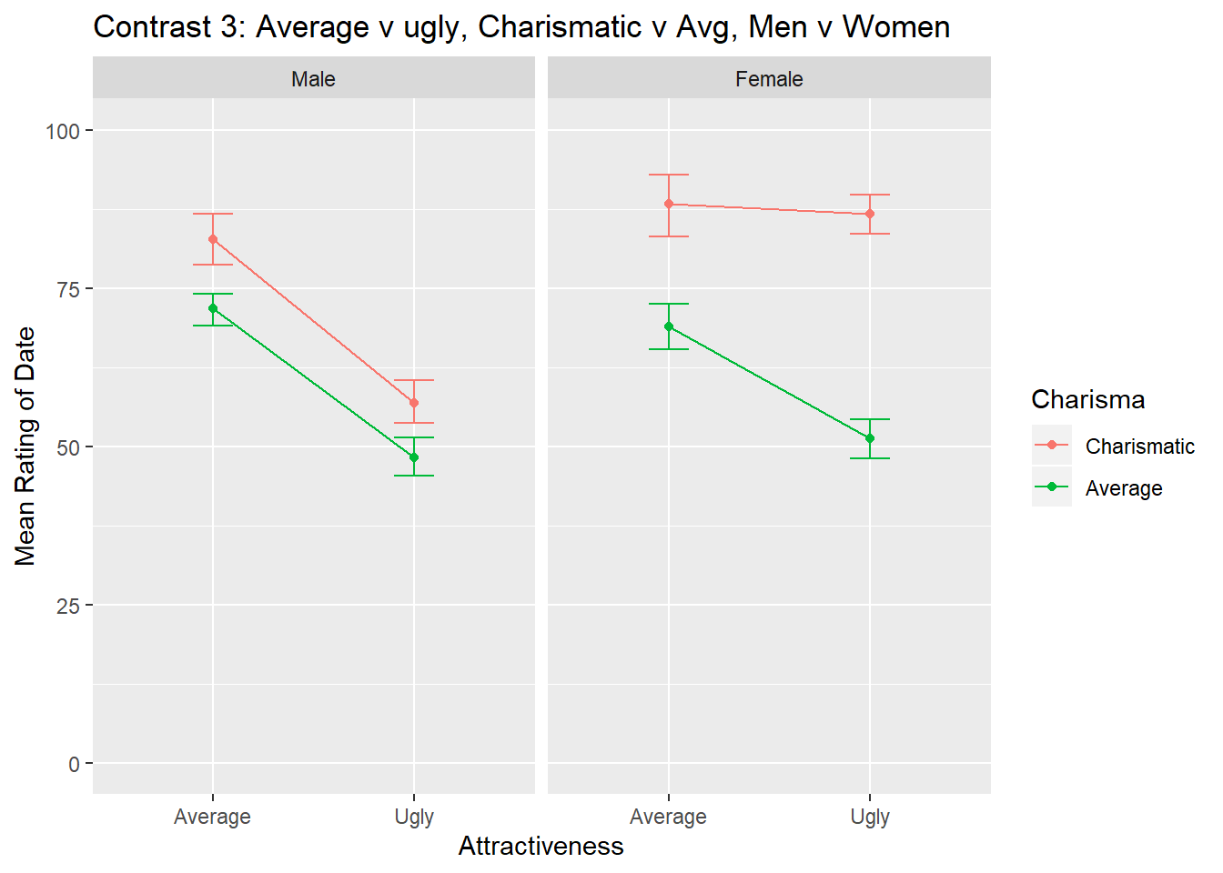
Contrast 3 compares whether interest in average versus ugly dates for high versus average charisma is different for men versus women. Again we can see that there is different pattern of results for men versus women. For men, as attractiveness decreases, so too do ratings of the date for both high and average levels of charisma. For women, when charisma is high, there is no change in ratings of the date based on attractiveness. However, when charisma is average looks matter, as there is a decrease in ratings of the date going from attractive to ugly.
contrast4 <- speed_long %>%
  filter(Personality=="Average" | Personality == "Dullard") %>%
  filter(Looks == "Average" | Looks == "Ugly") %>%
  ggplot(aes(Looks, Rating, color=Personality)) +
    stat_summary(fun.y = mean, geom = "point") +
    stat_summary(fun.y = mean, geom = "line", aes(group= Personality)) +
    stat_summary(fun.data = mean_cl_boot, geom = "errorbar", width = 0.2) +
    labs(x = "Attractiveness", y = "Mean Rating of Date", colour = "Charisma") +
    scale_y_continuous(limits = c(0,100)) +
    scale_color_manual(values = c("#00BA38", "#619CFF")) +
    facet_wrap(~Gender) +
    ggtitle("Contrast 4: Avg v Ugly, Avg v Dullard, Men v Women")
contrast4
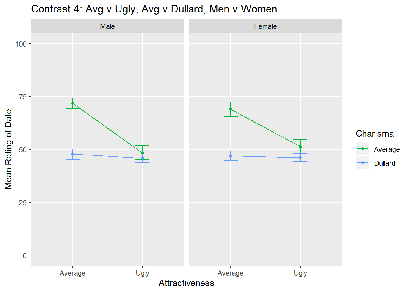 For contrast 4, we see the same pattern of results for men and women when comparing average v ugly for average v dullard, and thus this contrast is not statistically significant.