One-Way ANOVA
This week in class, we learned how to conduct a one-way ANOVA by hand using Excel. The instructions and exercises below will demonstrate how to run that same ANOVA in R. If you would like a copy of the Excel exercise, please email me at afox-galalis@mghihp.edu.
Packages you should have loaded to successfully run this week’s exercises: mosaic, dplyr, ggplot2, emmeans, ggsignif, car, ez, apaTables, DescTools, and MOTE.
Hopefully, you have successfully run the ANOVA “by hand” using Excel. For this exercise, we will bring the data into R and run the one-way ANOVA here. We will also conduct post-hoc tests to determine which groups are significantly different from one another. Before we run the ANOVA, practice running a power analysis in GPower for a one-way ANOVA.
Power Analysis
Using what you learned last week, see if you can conduct a power analysis on your own.
- A researcher is interested in examining whether background noise impairs learning retention. She designs a 4-condition experiment and will compare retention scores for participants randomized to a no noise, low noise, moderate noise, or high noise condition. Participants were only assigned to one group. How many participants will she need to achieve 80% power if she expects an overall medium effect size, with an alpha of .05? How many for a small effect size?
One-way ANOVA
First, let’s bring the data into R. We could cut and paste the data into an excel worksheet, save as a csv, and then import it. But because we have such a small dataset, this is another good opportunity to practice creating a dataframe in R. We will create a factor variable and then enter the data for each condition into a vector. Then we will merge everything into a dataframe.
group <- rep(1:3, each=10)  #Creating a variable that we will then factor
group <-factor(group, labels = c("vigorous", "moderate", "none"))  #factoring the variable
score <- c(20,15,18,14,19,18,20,15,14,17,11,10,8,10, 13,12,11,15,16,14,5,8,9,10,12,10,6,5,8,7)  #entering the data; scores are entered for the vigorous group, then the moderate group and finally the none group.

exercise <- data.frame(group, score)  #merging the two variables into a dataframe
exercise$id = 1:nrow(exercise)  #adding an ID#
Cleaning and Screening the data
After creating/entering the data, we should make sure that everything looks the way we expect. Look in your Environment to confirm that the exercise dataset now appears there, and that it has three variables: a factor variable called “group”, a numeric variable called “score”, and an ID variable.
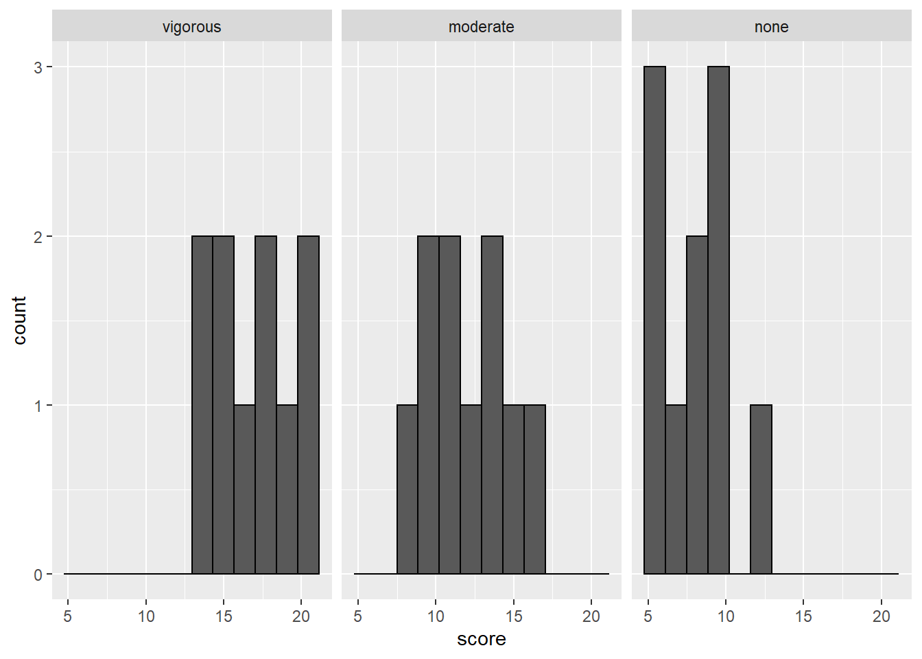
- Run descriptive statistics by group on the outcome variable. Then create a histogram for each group.
The code below demonstrates how to get the descriptives and the histograms:
#Descriptive statistics by group
favstats(score ~ group, data = exercise)
##      group min    Q1 median    Q3 max mean       sd  n missing
## 1 vigorous  14 15.00   17.5 18.75  20   17 2.357023 10       0
## 2 moderate   8 10.25   11.5 13.75  16   12 2.494438 10       0
## 3     none   5  6.25    8.0  9.75  12    8 2.309401 10       0
#histograms for each group using facet_wrap
exercise %>%
  ggplot(aes(x=score), fill=group) +
  geom_histogram(bins=12, color = "black") +
  facet_wrap(~group)
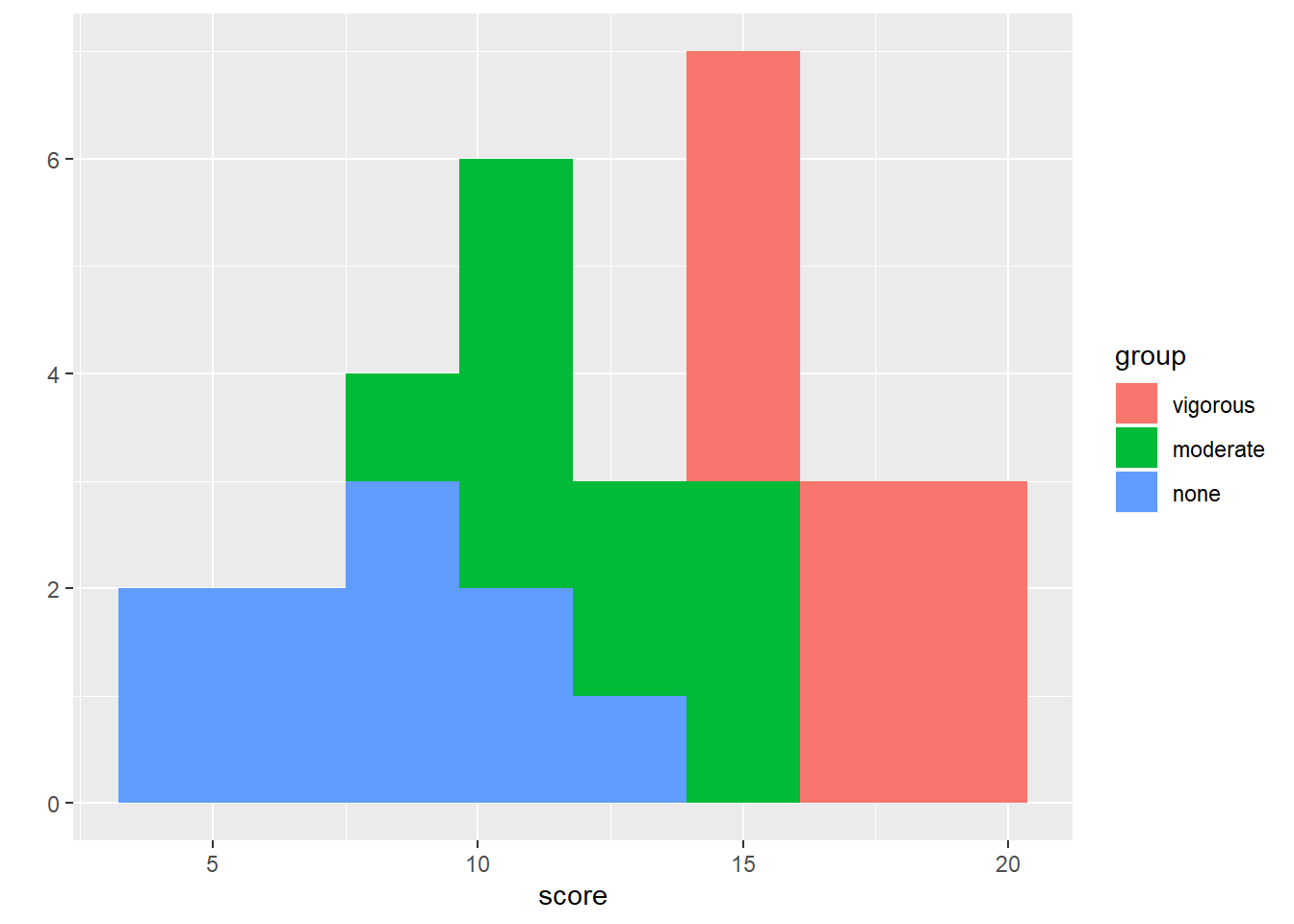
#histograms on same plot using qplot, using fill=group
qplot(x = score, fill = group, data = exercise, bins = 8)
boxplot(score ~ group,
        data = exercise,
        ylab="Score",
        xlab="Group")
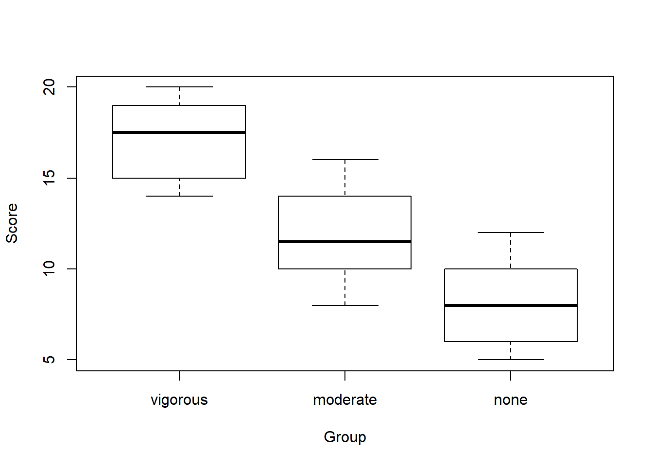
We don’t have any outliers or missing data with this dataset. We only have 10 cases per group, so the shapes of the histograms are not suprising. From the descriptive statistics, we can see that the means look like they are quite different from one another. The SDs are are also similar. To confirm we have met the assumption of homogeneity of variance, we can use Levene’s test like we did with the t-tests last week.
library(car)
leveneTest(score~group, data=exercise)
## Levene's Test for Homogeneity of Variance (center = median)
##       Df F value Pr(>F)
## group  2  0.0773 0.9259
##       27
Now we can go ahead and run the one-way ANOVA. As is the case with most analyses in R, there are several ways to run a one-wayANOVA. The first method is to use the aov function. Save the results of the analysis to an object, and then use summary to call the results.
options(scipen=999)  #turns off scientific notation
mod1 <- aov(score ~ group, data = exercise)  #running the anova model
summary.aov(mod1)  #printing the summary of results
##             Df Sum Sq Mean Sq F value       Pr(>F)
## group        2  406.7   203.3   35.65 0.0000000265 ***
## Residuals   27  154.0     5.7
## ---
## Signif. codes:  0 '***' 0.001 '**' 0.01 '*' 0.05 '.' 0.1 ' ' 1
- Based on the results of the ANOVA analysis, what can you conclude?
Another way we can conduct the one-way ANOVA is to use the ezANOVA function from the ez package. Install the package and attach the library. The benefit of ezANOVA is that it also includes an effect size measure, ges, which represents generalized eta squared. In a one-factor between subjects design, this effect size is partial eta squared (
library(ez)
mod2<- ezANOVA(data = exercise,  #dataset
        wid = id,                #id from the dataset
        between = group,         #the between subjects variable (the IV)
        dv = score,              #the dependent variable
        type = 3,                #type III sum of squares; consistent with SPSS
        detailed = TRUE,         #more info in the output
        return_aov=TRUE)         #will print out the sum of squares
print(mod2)                      #prints the output we saved to object `mod2`
## $ANOVA
##        Effect DFn DFd       SSn SSd         F                             p
## 1 (Intercept)   1  27 4563.3333 154 800.06494 0.000000000000000000001335264
## 2       group   2  27  406.6667 154  35.64935 0.000000026547020504976994535
##   p<.05       ges
## 1     * 0.9673544
## 2     * 0.7253270
##
## $`Levene's Test for Homogeneity of Variance`
##   DFn DFd       SSn  SSd          F         p p<.05
## 1   2  27 0.2666667 46.6 0.07725322 0.9258593
##
## $aov
## Call:
##    aov(formula = formula(aov_formula), data = data)
##
## Terms:
##                    group Residuals
## Sum of Squares  406.6667  154.0000
## Deg. of Freedom        2        27
##
## Residual standard error: 2.388243
## Estimated effects may be unbalanced
Creating an ANOVA Table
There may be occasions when you need to create an APA-formatted ANOVA table for a manuscript. The apaTables package will create APA-formatted tables and save them as word documents. You’ll need to install and attach the package before running the code below. The word document containing the table will be saved to your working directory.
library(apaTables)
#Table for aov output
apa_table<- apa.aov.table(mod1,
                          filename="Table1_APA.doc",
                          table.number=1)
print(apa_table)
##
##
## Table 1
##
## ANOVA results using score as the dependent variable
##
##
##    Predictor      SS df      MS      F    p partial_eta2 CI_90_partial_eta2
##  (Intercept) 2890.00  1 2890.00 506.69 .000
##        group  406.67  2  203.34  35.65 .000          .73         [.53, .80]
##        Error  154.00 27    5.70
##
## Note: Values in square brackets indicate the bounds of the 90% confidence interval for partial eta-squared
#table for ezANOVA output
apa_table<- apa.ezANOVA.table(mod2,
                              table.title = "One-Way ANOVA Table",
                              filename="Table1_ezAPA.doc",
                              table.number=1)
print(apa_table)
##
##
## Table 1
##
## One-Way ANOVA Table
##
##    Predictor df_num df_den  SS_num SS_den      F    p ges
##  (Intercept)      1     27 4563.33 154.00 800.06 .000 .97
##        group      2     27  406.67 154.00  35.65 .000 .73
##
## Note. df_num indicates degrees of freedom numerator. df_den indicates degrees of freedom denominator.
## SS_num indicates sum of squares numerator. SS_den indicates sum of squares denominator.
## ges indicates generalized eta-squared.
##
Post-hoc Tests, Orthogonal Contrasts, and Trend Analysis
The one-way ANOVA is an omnibus test. That means it tells us if there is an overall difference in the means of the different groups, but it does not tell us which means are different from one another. To determine which means are different, we need to conduct follow-up tests. The follow-up tests you select will depend on your apriori hypotheses regarding the differences between the groups.
If you do not have any apriori hypotheses and just want to know which groups are different from one another, you can use post-hoc t-tests. However, remember whenever conducting multiple t-tests, you inflate the Type I error rate. There are several adjustments you can make to adjust for multiple comparisons.
LSD: No adjustment is made.
Bonferroni: divides the alpha by the number of tests conducted; very conservative.
Holm: Stepwise procedure where p-values are ranked smallest to largest. For each p-value, the adjusted alpha is calculated with the formula below.
If the p-value is smaller than the adjusted alpha, the comparison is statistically significant. This procedure continues for each p-value until a non-significant p-value is obtained. All comparisons after that point are not significant.
- Tukey HSD: The difference between each pair of means is calculated. Then the difference between each pair of means is compared against the HSD, which is a critical value calculated with the formula below.
q is the Studentized Range Statistic which you have to look up using a table (often found in the back of statistics textbooks).
- Scheffe: Corrects alpha for both simple and complex comparisons; low power/conservative
We can use the pairwise.t.test function to request most of these post-hoc tests. We will need to use a different function for TukeyHSD.
#No adjustment
pairwise.t.test(exercise$score, exercise$group,
                paired = F,
                var.equal = T,
                p.adjust.method = "none")
##
## 	Pairwise comparisons using t tests with pooled SD
##
## data:  exercise$score and exercise$group
##
##          vigorous     moderate
## moderate 0.0000717052 -
## none     0.0000000049 0.00087
##
## P value adjustment method: none
#Bonferroni
pairwise.t.test(exercise$score, exercise$group,
                paired = F,
                var.equal = T,
                p.adjust.method = "bonferroni")
##
## 	Pairwise comparisons using t tests with pooled SD
##
## data:  exercise$score and exercise$group
##
##          vigorous    moderate
## moderate 0.00022     -
## none     0.000000015 0.00260
##
## P value adjustment method: bonferroni
#Holm
pairwise.t.test(exercise$score, exercise$group,
                paired = F,
                var.equal = T,
                p.adjust.method = "holm")
##
## 	Pairwise comparisons using t tests with pooled SD
##
## data:  exercise$score and exercise$group
##
##          vigorous    moderate
## moderate 0.00014     -
## none     0.000000015 0.00087
##
## P value adjustment method: holm
#Tukey
TukeyHSD(mod1)
##   Tukey multiple comparisons of means
##     95% family-wise confidence level
##
## Fit: aov(formula = score ~ group, data = exercise)
##
## $group
##                   diff        lwr       upr     p adj
## moderate-vigorous   -5  -7.648154 -2.351846 0.0002059
## none-vigorous       -9 -11.648154 -6.351846 0.0000000
## none-moderate       -4  -6.648154 -1.351846 0.0024145
The DescTools package is also great for post-hoc tests.
#DescTools package

library(DescTools)

PostHocTest(mod1, method = "scheffe", conf.level = 0.95)
##
##   Posthoc multiple comparisons of means : Scheffe Test
##     95% family-wise confidence level
##
## $group
##                   diff     lwr.ci    upr.ci        pval
## moderate-vigorous   -5  -7.766295 -2.233705     0.00033 ***
## none-vigorous       -9 -11.766295 -6.233705 0.000000028 ***
## none-moderate       -4  -6.766295 -1.233705     0.00352 **
##
## ---
## Signif. codes:  0 '***' 0.001 '**' 0.01 '*' 0.05 '.' 0.1 ' ' 1
PostHocTest(mod1, method = "lsd", conf.level = 0.95)
##
##   Posthoc multiple comparisons of means : Fisher LSD
##     95% family-wise confidence level
##
## $group
##                   diff     lwr.ci    upr.ci         pval
## moderate-vigorous   -5  -7.191467 -2.808533 0.0000717052 ***
## none-vigorous       -9 -11.191467 -6.808533 0.0000000049 ***
## none-moderate       -4  -6.191467 -1.808533      0.00087 ***
##
## ---
## Signif. codes:  0 '***' 0.001 '**' 0.01 '*' 0.05 '.' 0.1 ' ' 1
PostHocTest(mod1, method = "bonferroni", conf.level = 0.95)
##
##   Posthoc multiple comparisons of means : Bonferroni
##     95% family-wise confidence level
##
## $group
##                   diff     lwr.ci    upr.ci        pval
## moderate-vigorous   -5  -7.726166 -2.273834     0.00022 ***
## none-vigorous       -9 -11.726166 -6.273834 0.000000015 ***
## none-moderate       -4  -6.726166 -1.273834     0.00260 **
##
## ---
## Signif. codes:  0 '***' 0.001 '**' 0.01 '*' 0.05 '.' 0.1 ' ' 1
Finally, you can use the emmeans package to conduct the contrasts and comparisons. This is my “go to” package for pairwise comparisons and contrasts. If you don’t already have the package installed, go ahead and install it.
library(emmeans)
emmeans(mod1, pairwise~group, adjust="tukey")  #can change to "bonferroni", "holm", "none"
## $emmeans
##  group    emmean    SE df lower.CL upper.CL
##  vigorous     17 0.755 27    15.45    18.55
##  moderate     12 0.755 27    10.45    13.55
##  none          8 0.755 27     6.45     9.55
##
## Confidence level used: 0.95
##
## $contrasts
##  contrast            estimate   SE df t.ratio p.value
##  vigorous - moderate        5 1.07 27 4.681   0.0002
##  vigorous - none            9 1.07 27 8.427   <.0001
##  moderate - none            4 1.07 27 3.745   0.0024
##
## P value adjustment: tukey method for comparing a family of 3 estimates
There may be situations in which we want to make specific comparisons or contrasts after finding a significant ANOVA. For example, we might first want to compare the two exercise conditions (vigorous + moderate) versus the no exercise condition. And after looking at that contrast, we could then look at moderate versus vigorous exercise comparison. These are orthogonal contrasts. See the Field book or this week’s PowerPoint notes for more detail about the rules for orthogonal contrasts.
To set up the contrasts in R, we need to tell R which groups we want to compare. Our groups are ordered as “vigorous”, “moderate”, “none”. This is important to know when setting up the contrasts. The coefficients for the contrasts should add to 1. If a group is not involved in the contrast, it is given a coefficient of 0.
#determine the order of the levels for your grouping variable
levels(exercise$group)
## [1] "vigorous" "moderate" "none"
#set up the contrasts
c1 <- c(-1,-1,2)  #exercise versus no exercise
c2 <- c(-1,1,0)   #vigorous versus moderate

# combined the above 2 lines into a matrix
mat <- cbind(c1,c2)

# tell R that the matrix gives the contrasts you want
contrasts(exercise$group) <- mat

# these lines give you your results
model1c <- aov(score ~ group, data = exercise)

#call the anova model with the contrasts
summary.aov(model1c, split=list(group=list("Exercise vs. No Exercise"=1, "Vigorous vs. Moderate" = 2)))
##                                   Df Sum Sq Mean Sq F value       Pr(>F)
## group                              2  406.7   203.3   35.65 0.0000000265 ***
##   group: Exercise vs. No Exercise  1  281.7   281.7   49.38 0.0000001486 ***
##   group: Vigorous vs. Moderate     1  125.0   125.0   21.92 0.0000717052 ***
## Residuals                         27  154.0     5.7
## ---
## Signif. codes:  0 '***' 0.001 '**' 0.01 '*' 0.05 '.' 0.1 ' ' 1
- Summarize the findings from the contrasts you examined.
Finally, we might be interested in examining whether there is a linear or quadratic trend present in the the data. Trend analyses are only appropriate when there is an ordering to the group variable. Further, the groups should be ordered in a meaningful way–smallest to largest, largest to smallest, etc., in order for the results of the trend analysis to make sense. With three groups, we can test a linear and quadratic trend. If we had 4 groups, we could also test a cubic trend.
Below I’ll show you how to do this manually and using functions in the emmeans package.
#setting the contrasts manually
contrasts(exercise$group)<-contr.poly(3)
model1d <- aov(score~group, data=exercise)
summary.aov(model1d, split=list(group=list("Linear"=1, "Quadratic"=2)))
##                    Df Sum Sq Mean Sq F value        Pr(>F)
## group               2  406.7   203.3  35.649 0.00000002655 ***
##   group: Linear     1  405.0   405.0  71.006 0.00000000488 ***
##   group: Quadratic  1    1.7     1.7   0.292         0.593
## Residuals          27  154.0     5.7
## ---
## Signif. codes:  0 '***' 0.001 '**' 0.01 '*' 0.05 '.' 0.1 ' ' 1
#With emmeans package
means_mod2 <-emmeans(mod2$aov, "group")   #first need to save the emmeans to an object
contrast(means_mod2, "poly")  #then can use the contrast function with "poly"
##  contrast  estimate   SE df t.ratio p.value
##  linear          -9 1.07 27 -8.427  <.0001
##  quadratic        1 1.85 27  0.541  0.5932
- Summarize the findings from your trend analysis of the exercise data.
One-way ANOVA with Unequal Variances
If Levene’s test is significant, and/or the largest group variance is more than twice as large as the smallest variance (some people use 4x instead of 2x), then you can use the Welch test to adjust for unequal variances.
oneway.test(score ~ group, data = exercise)
##
## 	One-way analysis of means (not assuming equal variances)
##
## data:  score and group
## F = 35.954, num df = 2.000, denom df = 17.982, p-value = 0.0000005206
Calculating Effect Sizes
The ezANOVA package provided the partial eta-squared effect size for a one-way between subjects ANOVA. But often, the overall effect size for the ANOVA is not the most interesting. The effect sizes for the pairwise comparisons are what we are really interested in. To calculate effect sizes for the pairwise comparisons from our ANOVA analysis, we will use aMOTE which was introduced last week. We will need the M/SD for each group. We can scroll back up to our previous descriptive statistics or we can just call them again. Below, we’ll use the pipe and dplyr to get the descriptive statistics.
library(MOTE)

exercise %>%
  group_by(group) %>%
  summarize(mean = mean(score, na.rm = TRUE),
            sd = sd(score, na.rm = TRUE),
            n = n())
## # A tibble: 3 x 4
##   group     mean    sd     n
##   <fct>    <dbl> <dbl> <int>
## 1 vigorous    17  2.36    10
## 2 moderate    12  2.49    10
## 3 none         8  2.31    10
Now that we have the descriptive statistics easily accessible in the table above, we can use MOTE to calculate the effect sizes for our three pairwise comparisons. We will calculate Cohen’s d for independent groups using the pooled SD.
The structure of d.ind.t is: d.ind.t(m1, m2, sd1, sd2, n1, n2, a = 0.05)
d.ind.t(17, 12, 2.36, 2.49, 10, 10, a = 0.05)$estimate
## [1] "$d_s$ = 2.06, 95\\% CI [0.94, 3.15]"
d.ind.t(17, 8, 2.36, 2.31, 10, 10, a =.05)$estimate
## [1] "$d_s$ = 3.85, 95\\% CI [2.31, 5.36]"
d.ind.t(12, 8, 2.49, 2.36, 10, 10, a = .05)$estimate
## [1] "$d_s$ = 1.65, 95\\% CI [0.61, 2.66]"
- Try running the effect size calculations without the $estimate at the end. What else could we request from the effect size output?
Plotting the Means with Error Bars
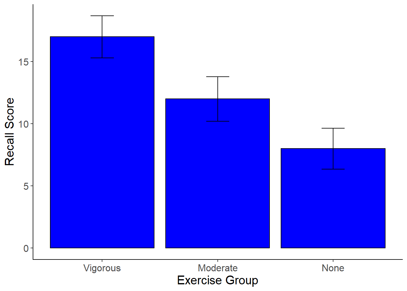
The next step of the analysis for a one-way ANOVA is to plot the means with error bars.
- Using ggplot2, create a bar graph of the means of each group. Include error bars, as well as axis titles and a title for the figure.
Here is what you graph should look like:
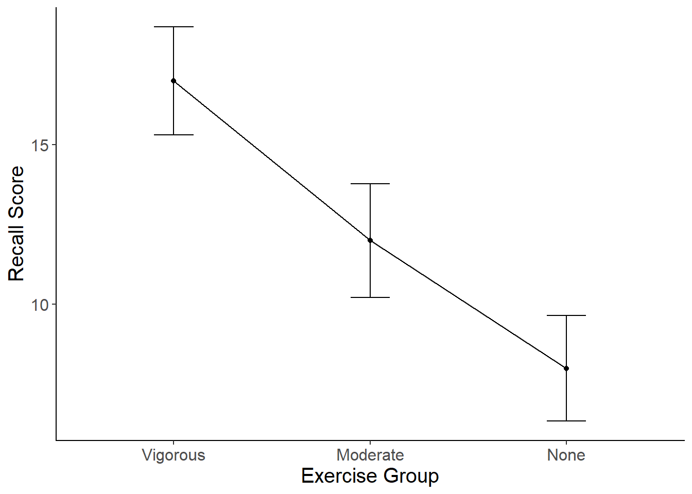
To make a line graph of your means:
mean_plot2 <-ggplot(data=exercise, aes(x = group , y = score)) +
  stat_summary(fun.y = mean,
               geom = "point") +
  stat_summary(fun.y = mean,
               geom = "line", aes(group=1)) +
  stat_summary(fun.data = mean_cl_normal,
               geom = "errorbar",
               width = .2,
               position = "dodge")  +
  xlab("Exercise Group") +
  ylab("Recall Score") +
  scale_x_discrete(labels = c("Vigorous","Moderate", "None")) +
  cleanup
mean_plot2
- Write up the results of the one-way ANOVA in an APA-formatted paragraph, including post-hoc tests (Tukey), effect sizes, and the graph of the means.
Non-parametric One-Way ANOVA
If you have a small sample, the data are not normally distributed, or you are not meeting the assumptions of a one-way ANOVA, you can instead use a non-parametric version of a one-way between subjects ANOVA. The Kruskal Wallis test is the non-parametric counterpart to a one-way ANOVA.
As with the non-parametric t-tests, the analysis is performed on ranked data.
kruskal.test(score ~ group, data = exercise)
##
## 	Kruskal-Wallis rank sum test
##
## data:  score by group
## Kruskal-Wallis chi-squared = 21.17, df = 2, p-value = 0.00002529
pairwise.wilcox.test(exercise$score, exercise$group,
                 p.adjust.method = "bonferroni")
##
## 	Pairwise comparisons using Wilcoxon rank sum test
##
## data:  exercise$score and exercise$group
##
##          vigorous moderate
## moderate 0.00488  -
## none     0.00053  0.01152
##
## P value adjustment method: bonferroni
The pairwise.wilcox.test code runs Mann-Whitney U t-tests as the post-hoc method. You can change the p.adjust.method to your preferred correction (e.g., Holm, BH, none). When you write up the results of a non-parametric ANOVA, instead of reporting the means and standard deviations, you should report the median (or mean rank).
On Your Own
Use the superhero.csv dataset available on the Field textbook companion website to run a one-way ANOVA with post-hoc tests and a graph of the means. Write a summary paragraph in APA format.