Repeated Measures ANOVA
One-Way Repeated Measures ANOVA
You are the statistician for a team conducting a study examining whether 4 lists of words are similarly easy or difficult to understand. The word lists are standard audiology tools for assessing hearing. They are calibrated to be equally difficult to understand; however, the original calibration was performed with no noise in the background. The experimenter wished to determine whether the lists were still equally difficult to understand in the presence of a noisy background.
Participants age 20 to 40 with normal hearing listened to standard audiology tapes of 50 English words from 4 different lists at low volume with a noisy background. They repeated the words and were scored based on the number of correct perceptions of the words. The order of list presentation was randomized.
You can download a copy of the data here:Download Audiology Dataset.
Loading, Cleaning and Screening the Data
The data for this lab are saved in an SPSS file (.sav file). To load an SPSS dataset, use the haven package. Install the package in the console and then call it using library. Use the summary function to confirm that the data has loaded properly. Factor any cateogrical variables that need to be factored.
library(haven) #install this package first in the console
## Warning: package 'haven' was built under R version 3.6.2
audiology <- read_sav("audiology.sav")
summary(audiology)
##    SubjectID        gender               age            List1
##  Min.   : 1.00   Length:24          Min.   :20.00   Min.   :18.00
##  1st Qu.: 6.75   Class :character   1st Qu.:24.75   1st Qu.:28.00
##  Median :12.50   Mode  :character   Median :28.50   Median :32.00
##  Mean   :12.50                      Mean   :29.17   Mean   :32.75
##  3rd Qu.:18.25                      3rd Qu.:32.50   3rd Qu.:36.50
##  Max.   :24.00                      Max.   :43.00   Max.   :48.00
##      List2           List3           List4
##  Min.   :16.00   Min.   :14.00   Min.   :14.00
##  1st Qu.:21.50   1st Qu.:19.50   1st Qu.:19.50
##  Median :30.00   Median :25.00   Median :25.00
##  Mean   :29.67   Mean   :25.25   Mean   :25.58
##  3rd Qu.:36.00   3rd Qu.:32.00   3rd Qu.:30.50
##  Max.   :44.00   Max.   :38.00   Max.   :42.00
audiology <- audiology %>%
  mutate(gender = factor(gender,
                         levels =c("M", "F"),
                         labels = c("Male", "Female")))
Sphericity
We need to check to make sure that our data meet the assumptions of a repeated measures ANOVA. The key assumption for repeated measures is Sphericity.
The assumption of sphericity in repeated measures designs is that the variances in the difference between all possible combinations of conditions are equal. Violating this assumption can lead to bias in the results, and increase the likelihood of making a Type I error.
To determine if we meet the assumption of sphericity, we can use Maulchy’s Test of Sphericity. If the results of this test indicate that sphericity has been violated (p<.05), we can use apply an adjustment to the degrees of freedom in our model. If p>.05, we are fine to interpret the results as presented. Some researchers and statisticians use a p<.001 cut-off instead of p<.05. Because the general linear model is fairly robust to violations of assumptions, you can use a more liberal cut-off like p<.001.
Estimates of Sphericity
If Maulchy’s test is significant, we will need to use an adjustment to the degrees of freedom. The adjustment is based on the value of Epsilon (\(\epsilon\)\ = 1, then there is sphericity. The farther \(\epsilon\)\ departs from 1, the less sphericity there is. There are two different ways of calculating \(\epsilon\):
Greenhouse Geiser. Conservative, tends to underestimate \(\epsilon\)\ when \(\epsilon\)\ is close to 1
Huynh-Feldt. Liberal, tends to overestimate \(\epsilon\)
So which should you use? It depends on the value of \(\epsilon\). If \(\epsilon\)\ <.75, use GG, and when >.75, use HF (or GG, as they will likely be very similar at that point). Multiply the df of the model by these estimates to correct for the effects of sphericity.
We can get the results of Maulchy’s test and the GG/HF corrections when we run the ANOVA model using ezANOVA.
Correlations between measures
For repeated measures designs, it is important that our repeated measures are correlated with one another. Higher correlations will give you more power to detect significant effects. However, we do not want the repeated measures to be perfectly correlated (r = 1.00). Correlations greater than .99 will be problematic, because that means you have essentially measured the same thing twice.
audiology %>%
  select(List1, List2, List3, List4) %>%    #selecting only the 4 repeated measures variables
  cor(use = "pairwise.complete.obs")   #running a correlation
##           List1     List2     List3     List4
## List1 1.0000000 0.5986566 0.1478432 0.3919009
## List2 0.5986566 1.0000000 0.4580991 0.4194151
## List3 0.1478432 0.4580991 1.0000000 0.4923197
## List4 0.3919009 0.4194151 0.4923197 1.0000000
The code above will output a correlation matrix. The correlations we are interested in are above (or below) the diagonal (note that they are the same, so you don’t need to look at both). None of the correlations are close .99, and the largest correlation is about 0.60 (between List 1 and List 2). This correlation table will come in handy again later on when we want to run a power analysis in G*Power because the correlation between repeated measurements impacts statistical power.
Restructuring the data
Before we run the analysis, we need to restructure the data. The datset we have been working with is in “wide” format–meaning that each participant has one row, and all of the dependent measures have their own column. To conduct a repeated measures ANOVA in R, we need the data to be in “long” format. Each participant will have multiple rows of data. Below are two methods that you can use to restructure the data. The first method uses the package reshape2 and the melt function. All of the variables that you want to keep in the dataset go on the id line. The variables that you want to combine go on the measured line. Any variables that are not included on either the id or measured lines are dropped from the dataset.
The second (and preferred) method is to use the gather function from tidyr. The key variable is the variable that will identify which measurement that row corresponds to (List 1, List 2, etc.), and the value represents the actual measurements. Variables that are not put on either of these lines will remain in the dataset. In the example below, I’ve also combined the restructuring of the data with factoring of the categorical variables (including the new List variable).
#Method 1: Using reshape2
library(reshape2)
temp_aud <-melt(audiology,
                id = c("SubjectID","gender", "age"),
                measured = c("List1", "List2", "List3", "List4"))
#Method 2: Using dplyr
audiology_long <- audiology %>%
  gather(key = "List", value = "Score", List1:List4) %>%
  mutate(List = factor(List, labels = c("List 1", "List 2", "List 3", "List 4")))
## Warning: attributes are not identical across measure variables;
## they will be dropped
audiology_long <- audiology_long %>%
  arrange(SubjectID)
Running a Repeated Measures ANOVA using ezANOVA
We are finally ready to run the analysis. We will call the ez package, and then use ezANOVA to run the analysis. We will use the new restructured dataset that we created above. The dv is Score, our within subjects id (wid) is SubjectID and our within subjects independent variable is List. We will use type=3 to get the Type III sums of squares, and include detailed = TRUE to get the full ANOVA output (including SS values).
library(ez)
## Warning: package 'ez' was built under R version 3.6.2
Model<-ezANOVA(data = audiology_long,
               dv = .(Score),
               wid = .(SubjectID),
               within = .(List),
               type = 3,
               detailed = TRUE,
               return_aov = TRUE)
## Warning: Converting "SubjectID" to factor for ANOVA.
print(Model)
## $ANOVA
##        Effect DFn DFd        SSn      SSd          F            p p<.05
## 1 (Intercept)   1  23 76953.3750 3231.625 547.689669 1.534027e-17     *
## 2        List   3  69   920.4583 2506.542   8.446116 7.412012e-05     *
##         ges
## 1 0.9306076
## 2 0.1382355
##
## $`Mauchly's Test for Sphericity`
##   Effect         W         p p<.05
## 2   List 0.7482825 0.2786423
##
## $`Sphericity Corrections`
##   Effect       GGe        p[GG] p[GG]<.05       HFe        p[HF] p[HF]<.05
## 2   List 0.8505496 0.0002084128         * 0.9656781 9.393003e-05         *
##
## $aov
##
## Call:
## aov(formula = formula(aov_formula), data = data)
##
## Grand Mean: 28.3125
##
## Stratum 1: SubjectID
##
## Terms:
##                 Residuals
## Sum of Squares   3231.625
## Deg. of Freedom        23
##
## Residual standard error: 11.8535
##
## Stratum 2: SubjectID:List
##
## Terms:
##                      List Residuals
## Sum of Squares   920.4583 2506.5417
## Deg. of Freedom         3        69
##
## Residual standard error: 6.027163
## Estimated effects may be unbalanced
#table for ezANOVA output
apa_table_ez<- apa.ezANOVA.table(Model,
                              table.title = "One-Way Repeated Measures ANOVA Table",
                              filename="Table1_RM_ezAPA.doc",
                              table.number=1)
print(apa_table_ez)
##
##
## Table 1
##
## One-Way Repeated Measures ANOVA Table
##
##    Predictor df_num df_den Epsilon   SS_num  SS_den      F    p ges
##  (Intercept)   1.00  23.00         76953.38 3231.62 547.69 .000 .93
##         List   2.55  58.69    0.85   920.46 2506.54   8.45 .000 .14
##
## Note. df_num indicates degrees of freedom numerator. df_den indicates degrees of freedom denominator.
## Epsilon indicates Greenhouse-Geisser multiplier for degrees of freedom,
## p-values and degrees of freedom in the table incorporate this correction.
## SS_num indicates sum of squares numerator. SS_den indicates sum of squares denominator.
## ges indicates generalized eta-squared.
##
We get two sets of output for the ezANOVA here. One is for Maulchy’s Test of Sphericity, the other is the main ANOVA model results. Remember if Maulchy’s test has a p>.05 (or p>.001), we can proceed with the interpretation of the main ANOVA results. In this example, Maulchy’s test is non-significant, so we won’t need to make any adjustments to the main ANOVA findings.
From the ANOVA table, we can see that there is a main effect of List, F(3,69) = 8.45, p<.001, \(\eta^2\)\ = .14. Like the between subjects one-way ANOVA we did earlier this semester, this F-test is an omnibus one. When p<.05, we can conclude that at least two of our means are different. We will need to do post-hoc tests to determine which means are actually different.
Post-hoc Tests to Explore the Significant Main Effect
With a one-way repeated measures ANOVA, the easiest route for conducting follow-up testing is to examine all pairwise combinations of means.
First lets take a look at the means, standard deviations, and *n*s for each group (this will come in handy when we need to calculate effect sizes as well!). Then we can run pairwise t-tests using a bonferroni adjustment.
means <- audiology_long %>%
  group_by(List) %>%
  summarise(mean = mean(Score),
            sd = sd(Score),
            n = n())
means
## # A tibble: 4 x 4
##   List    mean    sd     n
##   <fct>  <dbl> <dbl> <int>
## 1 List 1  32.8  7.41    24
## 2 List 2  29.7  8.06    24
## 3 List 3  25.2  8.32    24
## 4 List 4  25.6  7.78    24
pairwise_ts <-pairwise.t.test(audiology_long$Score, audiology_long$List,
                paired = TRUE,
                p.adjust.method = "bonferroni")
pairwise_ts
##
## 	Pairwise comparisons using paired t tests
##
## data:  audiology_long$Score and audiology_long$List
##
##        List 1 List 2 List 3
## List 2 0.2422 -      -
## List 3 0.0097 0.1103 -
## List 4 0.0021 0.1687 1.0000
##
## P value adjustment method: bonferroni
The output from our pairwise comparisons is a table of p-values. From this table, we can see that List 1 is significantly different from List 3 (p = .01) and List 4 (p = .002) using a Bonferroni adjustment to the p-values.
Calculating Effect Sizes
To calculate the effect sizes for our pairwise comparisons, we will use the MOTE package.
library(MOTE)

#List 1 v List 2
onevtwo <- d.dep.t.avg(32.8, 29.7, 7.41, 8.06, 24, a = .05)

#List 1 v List 3
onevthreee <- d.dep.t.avg(32.8, 25.2, 7.41, 8.32, 24, a = .05)
onevthreee
## $d
## [1] 0.9663064
##
## $dlow
## [1] 0.4721963
##
## $dhigh
## [1] 1.446151
##
## $M1
## [1] 32.8
##
## $sd1
## [1] 7.41
##
## $se1
## [1] 1.51256
##
## $M1low
## [1] 29.67103
##
## $M1high
## [1] 35.92897
##
## $M2
## [1] 25.2
##
## $sd2
## [1] 8.32
##
## $se2
## [1] 1.698313
##
## $M2low
## [1] 21.68677
##
## $M2high
## [1] 28.71323
##
## $n
## [1] 24
##
## $df
## [1] 23
##
## $estimate
## [1] "$d_{av}$ = 0.97, 95\\% CI [0.47, 1.45]"
#List 1 v List 4
onevfour <-d.dep.t.avg(32.8, 25.6, 7.41, 7.78, 24, a = .05)
onevfour
## $d
## [1] 0.9479921
##
## $dlow
## [1] 0.4569131
##
## $dhigh
## [1] 1.424909
##
## $M1
## [1] 32.8
##
## $sd1
## [1] 7.41
##
## $se1
## [1] 1.51256
##
## $M1low
## [1] 29.67103
##
## $M1high
## [1] 35.92897
##
## $M2
## [1] 25.6
##
## $sd2
## [1] 7.78
##
## $se2
## [1] 1.588086
##
## $M2low
## [1] 22.31479
##
## $M2high
## [1] 28.88521
##
## $n
## [1] 24
##
## $df
## [1] 23
##
## $estimate
## [1] "$d_{av}$ = 0.95, 95\\% CI [0.46, 1.42]"
#List 2 v List 3
twovthree <- d.dep.t.avg(29.7, 25.2, 8.06, 8.06, 24, a = .05)

#List 2 v List 4
twovfour <- d.dep.t.avg(29.7, 25.6, 8.06, 7.78, 24, a = .05)

#List 3 v List 4
threevfour <- d.dep.t.avg(25.2, 25.6, 8.32, 7.78, 24, a = .05)
Plotting the Means
Finally, create a plot of the means with error bars using ggplot2. This is the same code we have been using the past few weeks, just modified for the present example.
library(ggplot2)
cleanup = theme(panel.grid.major = element_blank(),
panel.grid.minor = element_blank(),
panel.background = element_blank(),
axis.line = element_line(colour = "black"),
legend.key = element_rect(fill = "white"),
text = element_text(size = 15))
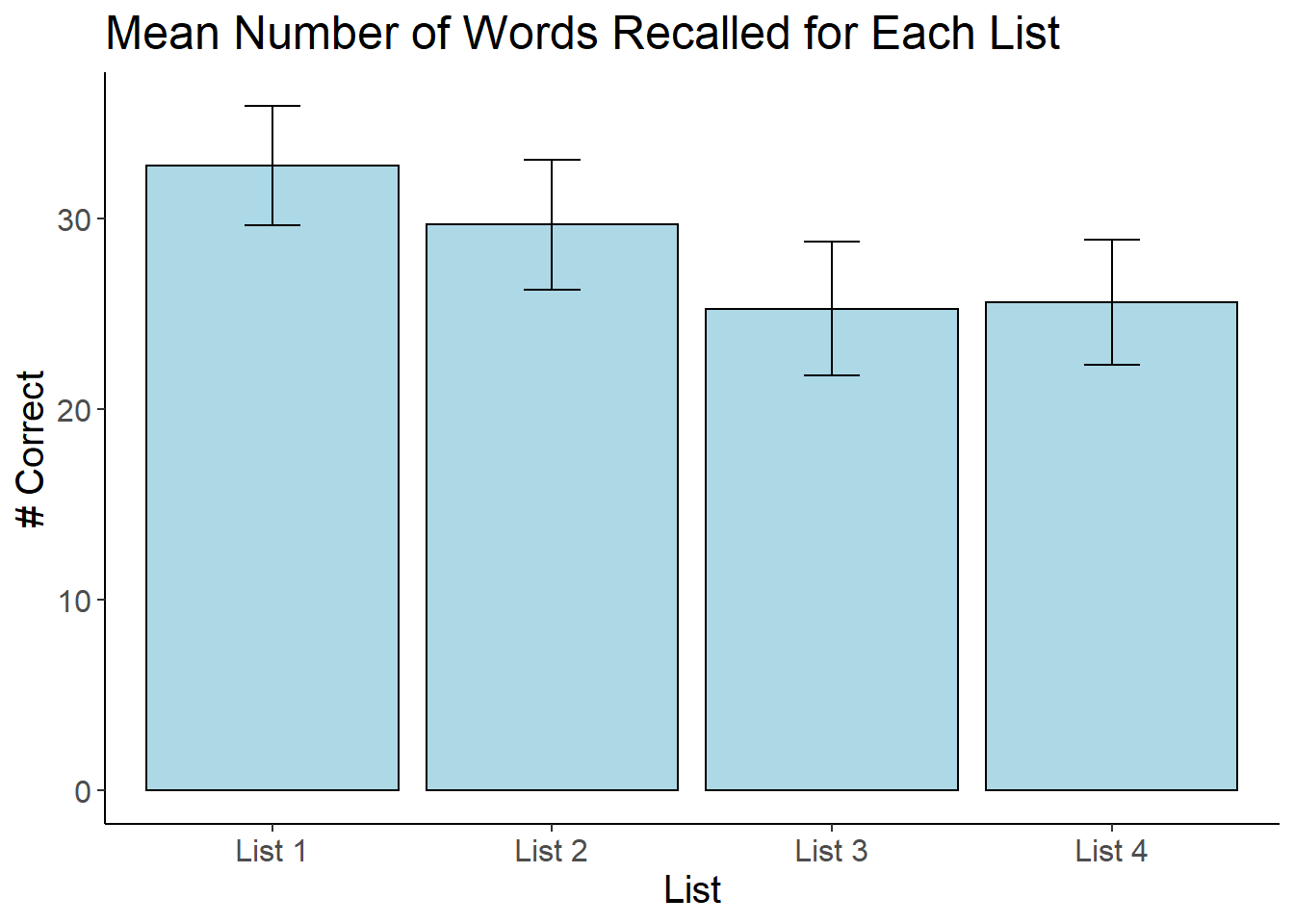
bargraph = ggplot(audiology_long, aes(x=List, y = Score))
bargraph +
stat_summary(fun.y = mean,
geom = "bar",
fill = "Light Blue",
color = "Black") +
stat_summary(fun.data = mean_cl_normal,
geom = "errorbar",
position = position_dodge(width = 0.90),
width = 0.2) +
cleanup +
xlab("List") +
ylab("# Correct") +
scale_x_discrete(labels = c("List 1", "List 2", "List 3", "List 4")) +
ggtitle("Mean Number of Words Recalled for Each List")
Writing the results in APA Format
To determine if there were differences across the 4 lists in terms of the number of items recalled, a one-way repeated measures ANOVA was conducted. Maulchy’s Test of Sphericity was not statistically significant (p= 0.28). The main effect of list was statistically significant, F(3, 69) = 8.45, p< .001, \(\eta^2\) = .14. Figure 1 contains a graph of the means with 95% confidence intervals. Post-hoc t-tests with a Bonferonni correction were used to determine which means were different from one another. Words on List 1 (M =32.75), SD = 7.41) were remembered better than the words on List 3 (M = 25.25, SD = 8.32, \(d_{av}\) = 0.97, 95\% CI [0.47, 1.45]) and List 4 (M = 25.58, SD = 7.78, \(d_{av}\) = 0.95, 95\% CI [0.46, 1.42]). No other comparisons were statistically significant.
Power Analysis for a single factor repeated measures design
You can use G*Power to conduct a power analysis for a repeated measures ANOVA. You’ll need slightly different information than you needed for between subjects ANOVA.
Test Family: F-Test
Statistical Test: ANOVA: Repeated measures, within factors
Type of Power Analysis: A priori
Input parameters:
Effect size f: Click on “Determine” and then use an eta square you think might be accurate (can pull from pilot data)
alpha: .05
Power: .80
Number of groups:
Number of measurements: # of Levels
Corr among repeated measures: Pull smallest correlation from correlation table of the measures (e.g. pilot data)
Nonsphericity correction:
\(\epsilon\)\ ; Will need to estimate with pilot data, or just leave at the default
Once you input all of these parameters into G*Power, you can run the power analysis to see how many participants you would need for a study based on what you entered.
Non-parametric One-Way Repeated Measures: Friedman’s Test
The non-parametric version of a one-way repeated measures ANOVA is Friedman’s test. Similar to the other non-parametric tests we have covered so far this semester, Friedman’s test is also based on ranked data. The rank sums of each level of the IV are calculated, and then a F-statistic is calculated based on those sums.
To conduct the Friedman Test, we will need to install the PMCMRplus package. This package contains functions to run both the Friedman Test, as well as several different post-hoc tests shoud the overall ANOVA be statistically significant. Below is the code to run the Friedman test and then conduct post-hocs using the Conover Test. Explore the package documentation to see the other types of post-hocs that are available.
#using Base R
friedman.test(Score ~ List|SubjectID, data=audiology_long)
##
## 	Friedman rank sum test
##
## data:  Score and List and SubjectID
## Friedman chi-squared = 16.731, df = 3, p-value = 0.0008026
#using PMCMRplus package
library(PMCMRplus)
friedmanTest(audiology_long$Score, audiology_long$List, audiology_long$SubjectID)
##
## 	Friedman rank sum test
##
## data:  audiology_long$Score , audiology_long$List and audiology_long$SubjectID
## Friedman chi-squared = 16.731, df = 3, p-value = 0.0008026
#posthocs
frdAllPairsConoverTest(audiology_long$Score, audiology_long$List, audiology_long$SubjectID)
##
## 	Pairwise comparisons using Conover's all-pairs test for a two-way balanced complete block design
## data: audiology_long$Score , audiology_long$List and audiology_long$SubjectID
##        List 1  List 2  List 3
## List 2 0.51613 -       -
## List 3 0.00091 0.07642 -
## List 4 0.02195 0.44486 0.79655
##
## P value adjustment method: single-step
Two-Way Repeated Measures ANOVA
The above example only included one repeated measures independent variable, but it is possible to have multiple within subjects independent variables. This next example comes from the Field textbook. It involves a study examining the whether attitudes towards stimuli can be changed using positive imagery.
Summarized from Field pg 583-584:
Participants viewed a total of nine mock adverts over three sessions. In each session, they saw three advertisements for a brand of beer (Brain Death), a brand of wine (Dangleberry), and a brank of water (Puritan). Each advertisement was paired with either a negative, positive, or neutral image. The design was fully crossed–each type of drink was paired with each type of message for a total of 9 conditions. The order of presentation and the order of the sessions were randomized across participants.
After viewing each advertisement, participants were asked to rate the drinks on a scale ranging from −100 (dislike very much) through 0 (neutral) to 100 (like very much).
There are two independent variables: type of drink (beer, wine, water) and type of imagery (positive, negative, neutral).
attitudes <-read.delim("Attitude.dat", header = TRUE, fileEncoding = "UTF-8-BOM")

summary(attitudes)
##     beerpos         beerneg          beerneut      winepos
##  Min.   : 1.00   Min.   :-19.00   Min.   :-10   Min.   :11.00
##  1st Qu.:12.75   1st Qu.: -9.50   1st Qu.:  4   1st Qu.:22.25
##  Median :18.50   Median :  0.00   Median :  8   Median :25.00
##  Mean   :21.05   Mean   :  4.45   Mean   : 10   Mean   :25.35
##  3rd Qu.:31.00   3rd Qu.: 20.25   3rd Qu.: 16   3rd Qu.:29.25
##  Max.   :43.00   Max.   : 30.00   Max.   : 28   Max.   :38.00
##     wineneg          wineneut        waterpos       waterneg
##  Min.   :-23.00   Min.   : 0.00   Min.   : 6.0   Min.   :-20.0
##  1st Qu.:-15.25   1st Qu.: 6.00   1st Qu.:12.0   1st Qu.:-14.5
##  Median :-13.50   Median :12.50   Median :17.0   Median :-10.0
##  Mean   :-12.00   Mean   :11.65   Mean   :17.4   Mean   : -9.2
##  3rd Qu.: -6.75   3rd Qu.:16.50   3rd Qu.:21.0   3rd Qu.: -4.0
##  Max.   : -2.00   Max.   :21.00   Max.   :33.0   Max.   :  5.0
##    waterneut
##  Min.   :-13.00
##  1st Qu.:  0.00
##  Median :  2.50
##  Mean   :  2.35
##  3rd Qu.:  8.00
##  Max.   : 12.00
The dataset is in wide format, so we’ll need to restructure it before we proceed with the analysis. Restructuring this data is a bit more complicated than the previous example. Each column in the dataset actually contains information about both independent variables.
The first thing we will do that will make restructing easier is to rename the variables. We will use the “_” to create variable names that separate the two independent variables in each column name (one variable before the _ and the other variable after it). We also need to add an ID# to the dataset.
attitudes_temp <- attitudes %>%
  rename(beer_pos = beerpos,
         beer_neg = beerneg,
         beer_neut = beerneut,
         wine_pos = winepos,
         wine_neg = wineneg,
         wine_neut = wineneut,
         water_pos = waterpos,
         water_neg = waterneg,
         water_neut = waterneut) %>%
  mutate(id = row_number())
Now we can use tidyr to restructure the data. We’ve used gather before (when restructuring to graph means from a paired samples t-test). This function “gathers” up all of the variables you tell it to and puts them into one column. With the levels of two independent variables embedded in each column name, we then need to spread those out into separate columns. The separate function will do that for us, and we’ll tell R that the “_” separates the variables in the column names.
The last steps of the code rename the “value” variable that was created when we gathered the data, and then factor our independent variables.
attitudes_long <- attitudes_temp %>%
  gather(key = "key", value = "value", beer_pos:water_neut) %>%
  arrange(id) %>%
  separate(key, into = c("Drink", "Imagery"), sep = "_") %>%
  rename(Rating = value ) %>%
  mutate(Drink = factor(Drink,
                        levels = c("beer", "wine", "water"),
                        labels = c("Beer", "Wine", "Water")),
         Imagery = factor(Imagery,
                          levels = c("pos", "neg", "neut"),
                          labels = c("Positive", "Negative", "Neutral")))
Now we can run the ANOVA:
options(scipen=999)

attitudeModel<-ezANOVA(data = attitudes_long,
                       dv = .(Rating),
                       wid = .(id),
                       within = .(Drink, Imagery),
                       type = 3,
                       detailed = TRUE)
print(attitudeModel)
## $ANOVA
##          Effect DFn DFd       SSn      SSd          F                         p
## 1   (Intercept)   1  19 11218.006 1920.106 111.005411 0.00000000225532205754568
## 2         Drink   2  38  2092.344 7785.878   5.105981 0.01086293072949783174164
## 3       Imagery   2  38 21628.678 3352.878 122.564825 0.00000000000000002680197
## 4 Drink:Imagery   4  76  2624.422 2906.689  17.154922 0.00000000045890402815248
##   p<.05       ges
## 1     * 0.4126762
## 2     * 0.1158687
## 3     * 0.5753191
## 4     * 0.1411741
##
## $`Mauchly's Test for Sphericity`
##          Effect         W              p p<.05
## 2         Drink 0.2672411 0.000006952302     *
## 3       Imagery 0.6621013 0.024452301563     *
## 4 Drink:Imagery 0.5950440 0.435658665787
##
## $`Sphericity Corrections`
##          Effect       GGe                 p[GG] p[GG]<.05       HFe
## 2         Drink 0.5771143 0.0297686804863521587         * 0.5907442
## 3       Imagery 0.7474407 0.0000000000001757286         * 0.7968420
## 4 Drink:Imagery 0.7983979 0.0000000190024850184         * 0.9785878
##                    p[HF] p[HF]<.05
## 2 0.02881390952906696945         *
## 3 0.00000000000003142804         *
## 4 0.00000000068096395208         *
apa_table_2way<- apa.ezANOVA.table(attitudeModel,
                              table.title = "Two-Way Repeated Measures ANOVA Table",
                              filename="Table1_RM2_ezAPA.doc",
                              table.number=1,
                              correction = "GG")
print(apa_table_2way)
##
##
## Table 1
##
## Two-Way Repeated Measures ANOVA Table
##
##        Predictor df_num df_den Epsilon   SS_num  SS_den      F    p ges
##      (Intercept)   1.00  19.00         11218.01 1920.11 111.01 .000 .41
##            Drink   1.15  21.93    0.58  2092.34 7785.88   5.11 .030 .12
##          Imagery   1.49  28.40    0.75 21628.68 3352.88 122.56 .000 .58
##  Drink x Imagery   3.19  60.68    0.80  2624.42 2906.69  17.15 .000 .14
##
## Note. df_num indicates degrees of freedom numerator. df_den indicates degrees of freedom denominator.
## Epsilon indicates Greenhouse-Geisser multiplier for degrees of freedom,
## p-values and degrees of freedom in the table incorporate this correction.
## SS_num indicates sum of squares numerator. SS_den indicates sum of squares denominator.
## ges indicates generalized eta-squared.
##
First thing to note is Maulchy’s test, which indicates that the data violation the assumption of sphericity for both of the main effects. In both cases, the epsilon value is less than .75, so we will need to apply the GG adjustment to the degrees of freedom. One nice thing about the apa.ezANOVA.table function is that the table will include the GG adjustment to the degrees of freedom. Note that the p-values in the “Spericity Corrections” table indicate that the main effects are still significant (p=.30 and p<.001). These are the p-vlaues we will need to report when we write up the findings for the main effects.
From the results of the ANOVA table, we can see that there is a significant main effect of Drink, a significant main effect of Imagery, and a significant Drink x Imagery interaction. When you have a significant interaction, it supercedes the main effects. In fact, although you should report the significant main effects, you often don’t need to interpret them (because they are qualified by the interaction).
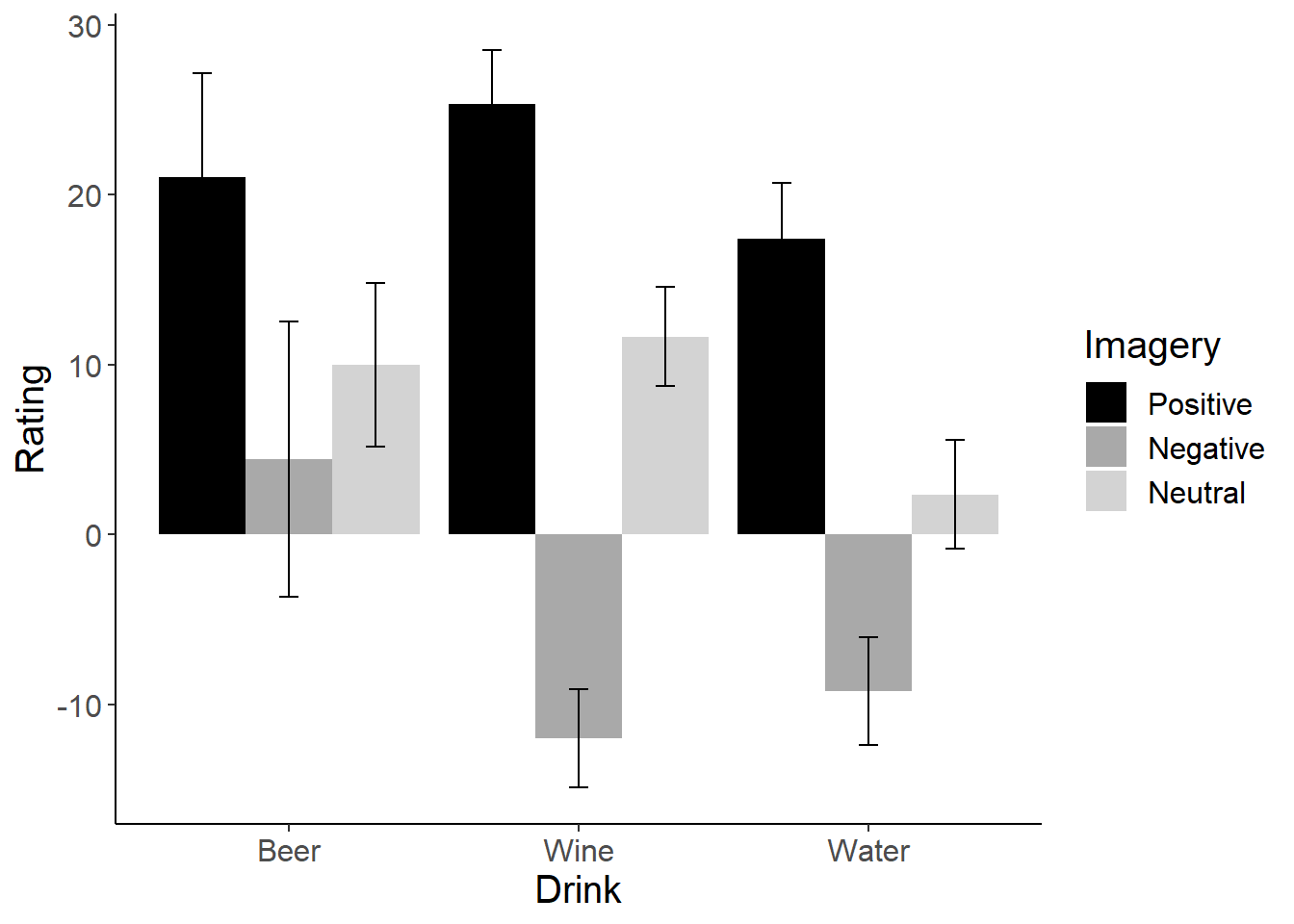
Our interaction is between two independent variables that each have 3 levels. We need to break that interaction down. Because we’d be doing the same number of tests regardless of how we decide to split up the interaction, let’s take a look at a graph of the interaction to see if we can figure out the best way to break it down (it would be better if we had a theoretical argument for how to break down the interaction, but we do not in this case). In the Field textbook, he calculates post-hoc t-tests for all 36 possible comparisons. This is overkill (in my opinion!).
# Bar Graph
attitude_graph = ggplot(attitudes_long, aes(x=Drink, y = Rating, fill=Imagery))
attitude_graph +
  stat_summary(fun.y = mean,
               geom = "bar",
               position = position_dodge(width=0.9)) +
  stat_summary(fun.data = mean_cl_normal,
               geom = "errorbar",
               width = 0.2,
              position = position_dodge(width=0.9)) +
  scale_fill_manual(values = c("black", "dark gray", "light gray"))+
  cleanup
#Line Graph
attitudeInt <- ggplot(attitudes_long, aes(x=Drink, y=Rating, colour = Imagery))
attitudeInt +
  stat_summary(fun.y = mean,
               geom = "point") +
  stat_summary(fun.y = mean,
               geom = "line",
               aes(group=Imagery)) +
  stat_summary(fun.data = mean_cl_boot,
               geom = "errorbar", width = 0.2) +
  labs(x = "Type of Drink", y = "Mean Attitude", colour = "Type of Imagery") +
  scale_colour_manual(values = c("navy", "light blue", "black")) +
  cleanup
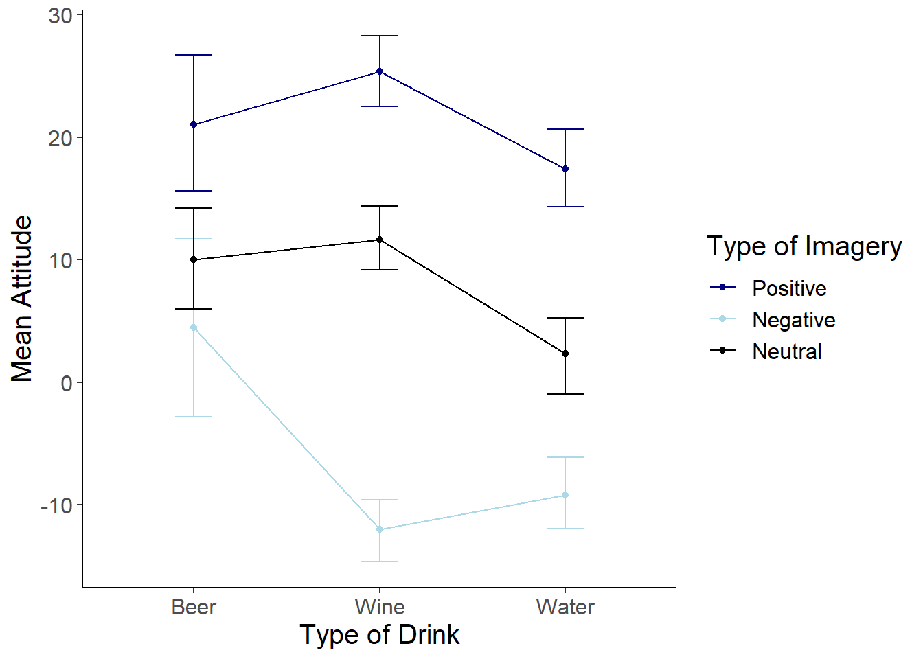
From the graph, it looks like there is something going on with the Beer group, so lets break down the interaction based on Drink. Subset the data into three mini-datasets–one for each level of Drink. Then, we’ll conduct pairwise t-tests within each of these groups.
In total, we will be doing 9 different t-tests, so if we want to adjust our p-values to avoid Type I error inflation, we’ll have to add a step to the process we have used in the past. When we use the pairwise.t.test function, we could set the adjustment method to “bonferroni”. The problem with this is that it thinks we are only doing 3 t-tests and will therefore adjust the p-values accordingingly. We really need to adjust to account for 9 tests. To do that, we will set the p.adjust.method to “none”. After we conduct our t-tests, we can then use the p.adjust function to get the corrected p-values.
beer_group<- subset(attitudes_long, Drink == "Beer")
wine_group <- subset(attitudes_long, Drink == "Wine")
water_group <- subset(attitudes_long, Drink == "Water")

pairwise.t.test(beer_group$Rating, beer_group$Imagery, p.adjust.method = "bonferroni", paired=TRUE)
##
## 	Pairwise comparisons using paired t tests
##
## data:  beer_group$Rating and beer_group$Imagery
##
##          Positive Negative
## Negative 0.00018  -
## Neutral  0.00165  0.13904
##
## P value adjustment method: bonferroni
pairwise.t.test(wine_group$Rating, wine_group$Imagery, p.adjust.method = "none", paired=TRUE)
##
## 	Pairwise comparisons using paired t tests
##
## data:  wine_group$Rating and wine_group$Imagery
##
##          Positive        Negative
## Negative 0.0000000000054 -
## Neutral  0.0000006211571 0.0000000063245
##
## P value adjustment method: none
pairwise.t.test(water_group$Rating, water_group$Imagery, p.adjust.method = "none", paired=TRUE)
##
## 	Pairwise comparisons using paired t tests
##
## data:  water_group$Rating and water_group$Imagery
##
##          Positive        Negative
## Negative 0.0000000000014 -
## Neutral  0.0000000248785 0.0000189413327
##
## P value adjustment method: none
#run the tests using "none" then adjust for bonferroni after the fact
p.adjust(.04635, method="bonferroni", n = 9)
## [1] 0.41715
Effect Size Calculations
Use the MOTE package to calculate effect sizes for the pairwise comparisons you conducted above. To make things a little easier, get the means, SDs, and ns for each group using the group_by and summarise functions.
library(MOTE)

attitudes_long %>%
  group_by(Drink, Imagery) %>%
  summarise(mean = mean(Rating),
            sd = sd(Rating),
            n = n())

#Beer: Positive v Negative
d.dep.t.avg(m1, m2, sd1, sd2, n, a = .05)$estimate

#Beer: Positive v Neutral
d.dep.t.avg(m1, m2, sd1, sd2, n, a = .05)

#Beer: Neutral v Negative
d.dep.t.avg(m1, m2, sd1, sd2, n, a = .05)