T-Tests
Independent Samples T-Tests
To learn how to conduct independent samples t-tests in R, we will use the smoking and health dataset. This study was designed to examine the relationship between health-related quality of life (HRQoL) and smoking in faculty, staff and students in a large department of nursing in a US university. The SF-36, V.2 was used for gathering data about HRQoL. The SF-36 contains 36 items that assess health in 8 domains throughout the past 4 weeks: physical function, role as it relates to physical function, bodily pain, general health perceptions, vitality, social function, role as it relates to emotional function, and mental health. Scores range from 0 to 100 for each domain. In addition to the SF-36, participants responded to supplemental questions about their health behaviors that were derived by the investigators.
The research question we need to answer is: Is there a difference in the general health of smokers versus non-smokers? What is the IV? What is the DV?
You can download the data for this exercise here: Download Smoking and Health Dataset
Cleaning and Screening the Data
smoking <- read_csv("smokinghealth.csv")
Because we are comparing two independent groups, we need to conduct an independent samples t-test. But before we get to the actual analysis, we need to clean and screen the data. Use the summary function to take a look at the two variables we will be using: smoking_status and general_health.
summary(smoking$smoking_status)
##    Length     Class      Mode
##      1258 character character
summary(smoking$general_health)
##    Min. 1st Qu.  Median    Mean 3rd Qu.    Max.    NA's
##    0.00   58.33   70.83   67.64   79.17  100.00       2
table(smoking$smoking_status)
##
##  currently smokes      never smoked previously smoked
##               143               815               286
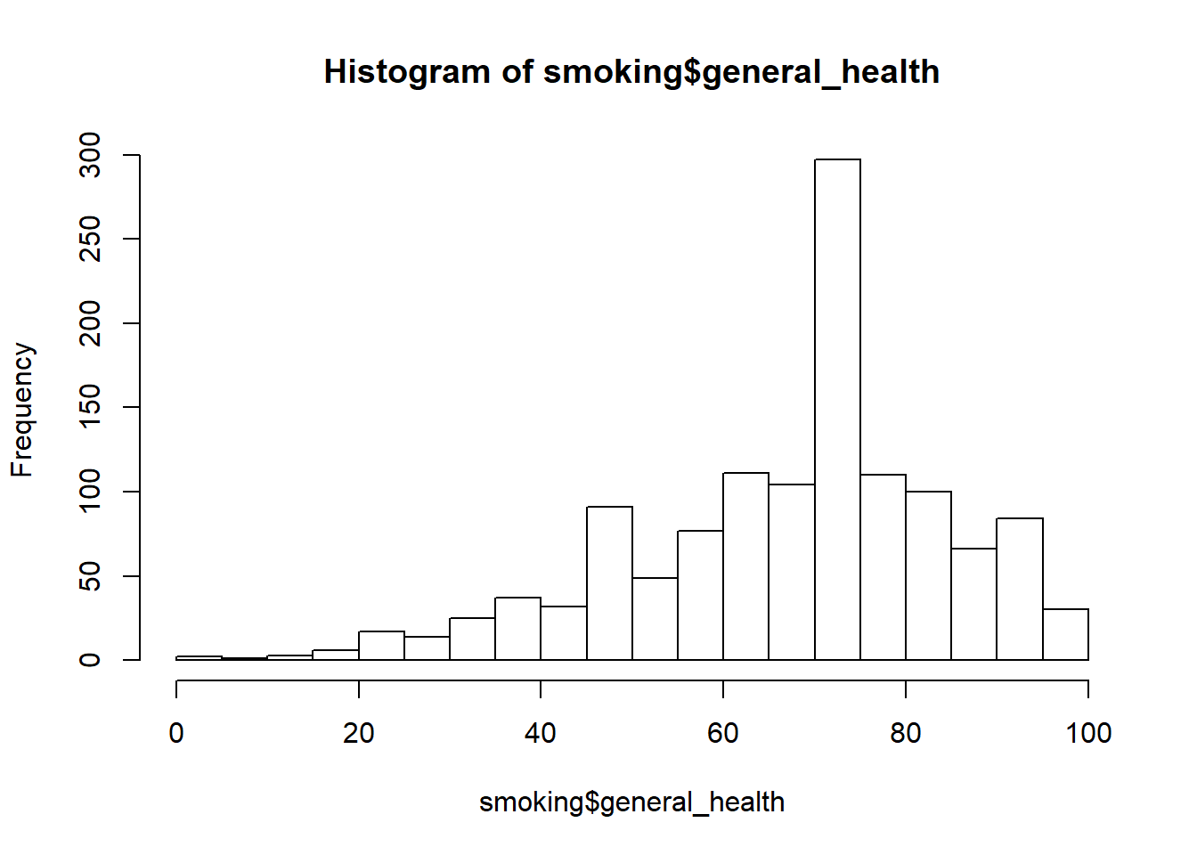
Our general_health variable looks good. The minimum and maximum scores (0 and 100) are within range for the variable, so there are no obvious errors we need to address.
We do have some issues with the smoking_status variable. First, the smoking_status variable is a character type variable, and we need it to be a factor. If we click on the dataset in the environment and look at the variable, we can see that it actually has three categories. To conduct a t-test, our IV can only have 2 levels, so we will need to fix that, too.
First, we will create a new variable where we combine those who have ever smoked with those who currently smoke. We will use the ifelse function from dplyr to do this.
Then, we will factor the new variable.
#recoding the smoking status variable into a dichotomous variable
smoking <- smoking %>%
  mutate(smoker = ifelse(smoking_status == "never smoked", "never smoked", "smoker"))

smoking <- smoking %>%
  mutate(smoker= as.factor(smoker))

table(smoking$smoker)
##
## never smoked       smoker
##          815          429
Now that we have created a new factor variable, we should double-check that the new variable is consistent with the old variable. The total of previous smokers plus current smokers should total the number of smokers in the new variable.
tally(~smoking_status, data=smoking) #looking at the Ns per group in the original variable
## smoking_status
##  currently smokes      never smoked previously smoked              <NA>
##               143               815               286                14
tally(~smoker, data=smoking) #looking at the Ns per group in the new variable
## smoker
## never smoked       smoker         <NA>
##          815          429           14
Everything seems to check out, so we can proceed with our data cleaning and screening. Note that we have missing data on our grouping variable (14 NAs). We can leave these in and drop them during analyses, or we can create another dataset that excludes those cases. For now, we will leave them in and deal with it as the need arises.
Note. If we were analyzing this dataset “for real”, we would do a full examination of missing data across people and variables and then have to make a determination about how to handle missingness. For the purpose of this lab, we are going to focus on the variables we are interested in.
Checking Assumptions
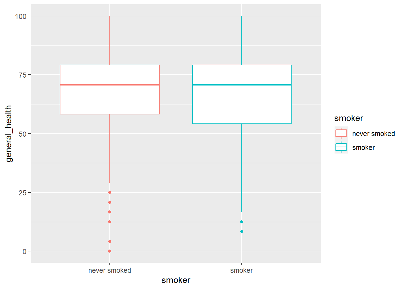
Next, we should look the boxplots and histograms for our dependent variable. Our sample size is large, so we don’t really need to worry about violating the assumption of normality. However, it is still good practice to take a look. We can examine the shape of the distribution, as well as check for any potential outliers. In addition to the histograms and boxplots, we can look at the skewness and kurtosis statistics using the describeBy function from the psych package.
#histogram of the entire sample
hist(smoking$general_health, breaks = 20)
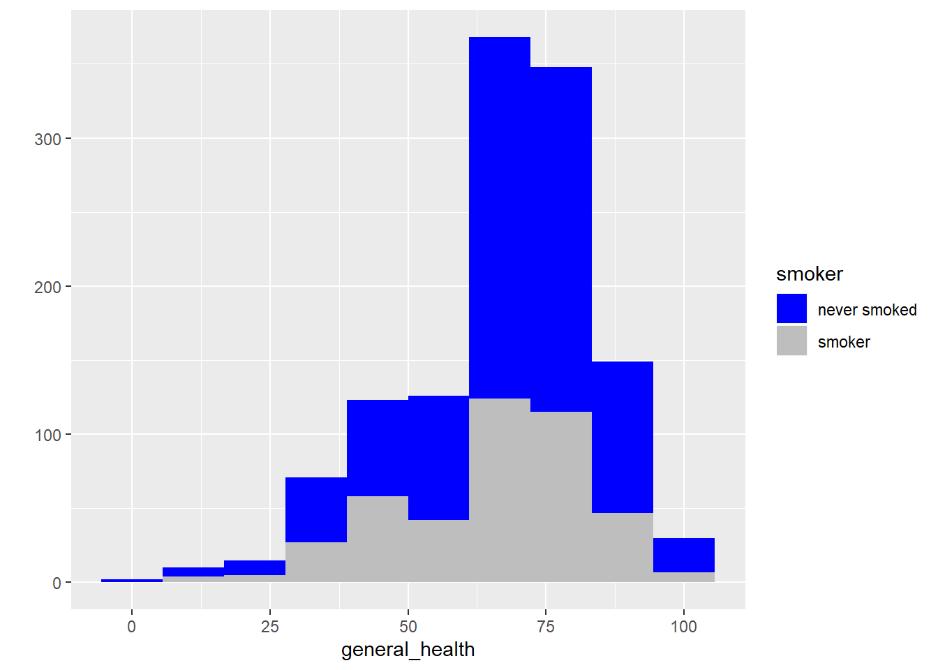
#histograms by group
qplot(x = general_health, fill = smoker, data = subset(smoking, !is.na(smoker)), bins = 10) +
  scale_fill_manual(values= c("blue", "gray"))
## Warning: Removed 2 rows containing non-finite values (stat_bin).
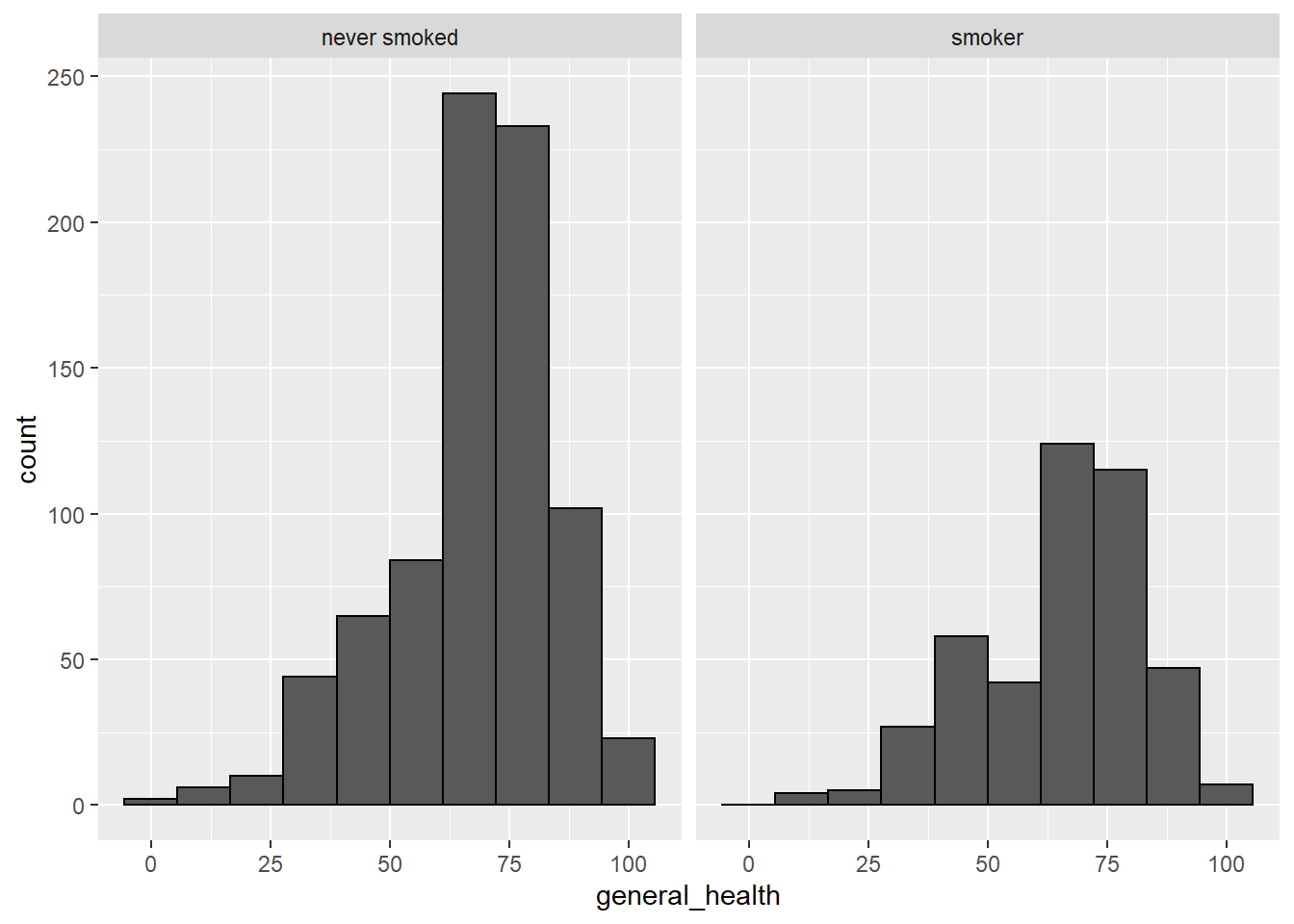
#another way to get histograms by group
smoking %>%
  dplyr::filter(!is.na(smoker)) %>%
  ggplot(aes(x=general_health), fill=smoker) +
  geom_histogram(bins=10, color = "black") +
  facet_wrap(~smoker)
## Warning: Removed 2 rows containing non-finite values (stat_bin).
#boxplots
qplot(y = general_health, x = smoker, color = smoker, data = subset(smoking, !is.na(smoker)), geom = "boxplot")
## Warning: Removed 2 rows containing non-finite values (stat_boxplot).
#descriptive statistics by group
describeBy(smoking$general_health, group=smoking$smoker)
##
##  Descriptive statistics by group
## group: never smoked
##    vars   n  mean    sd median trimmed   mad min max range skew kurtosis  se
## X1    1 813 68.67 17.21  70.83   70.09 18.53   0 100   100 -0.8     0.59 0.6
## ------------------------------------------------------------
## group: smoker
##    vars   n  mean    sd median trimmed   mad  min max range  skew kurtosis   se
## X1    1 429 66.16 17.29  70.83   67.29 18.53 8.33 100 91.67 -0.62     0.04 0.83
- Describe the shape of the distributions. Do the skewness and kurtosis values indicate a problem?
We can also check for outliers by using z-scores. Because we are going to be comparing two groups, we should calculate the z-scores within each group, rather than across the whole sample. We will use the group_by and mutate functions from dplyr to create the z-scores. We will then use the describeBy function to confirm that the mean and SD for each group are 0 and 1, respectively.
smoking <- smoking %>%
  group_by(smoker) %>%
  mutate(genhealthz = scale(general_health))
## Warning: Factor `smoker` contains implicit NA, consider using
## `forcats::fct_explicit_na`

## Warning: Factor `smoker` contains implicit NA, consider using
## `forcats::fct_explicit_na`
describeBy(smoking$genhealthz, group=smoking$smoker)
##
##  Descriptive statistics by group
## group: never smoked
##    vars   n mean sd median trimmed  mad   min  max range skew kurtosis   se
## X1    1 813    0  1   0.13    0.08 1.08 -3.99 1.82  5.81 -0.8     0.59 0.04
## ------------------------------------------------------------
## group: smoker
##    vars   n mean sd median trimmed  mad   min  max range  skew kurtosis   se
## X1    1 429    0  1   0.27    0.07 1.07 -3.35 1.96   5.3 -0.62     0.04 0.05
Now we need to make a decision about what to do about the cases that are greater than 3 SDs from the mean. Let’s go ahead and exclude them. Create a new dataset and only include those participants whose scores are less than 3 SD from the mean.
#How many cases have z-scores that are exceed +/- 3
sum(abs(smoking$genhealthz) >=3, na.rm=TRUE)
## [1] 10
table(smoking$genhealthz)
##
##  -3.99100778712197  -3.74883606899876  -3.34508512756556  -3.26449263275235
##                  1                  1                  1                  2
##  -3.10404751675435  -3.02232091462914  -2.86300990594314  -2.78014919650594
##                  1                  4                  2                  5
##  -2.62197229513193  -2.53797747838273  -2.38093468432072  -2.29580576025952
##                  2                  5                  3                  5
##   -2.1398970735095  -2.05363404213632   -1.8988594626983  -1.81146232401311
##                  9                 17                  7                 22
##  -1.65782185188708   -1.5692906058899  -1.51319928540036   -1.4277288620407
##                 11                 19                  1                  2
##  -1.41678424107587   -1.3271188877667  -1.17574663026466  -1.08494716964349
##                 13                 26                 17                 20
## -0.934709019453451 -0.882596023806981 -0.842775451520279 -0.721689592458678
##                 27                  1                 34                  1
## -0.700885077729072 -0.693671408642239 -0.600603733397076 -0.452633797831031
##                  3                 15                 49                 27
## -0.358432015273868 -0.337463185573258 -0.213128984399944 -0.211596187019819
##                 70                  1                  1                 38
## -0.116260297150659 -0.066973620533092 0.0294414237913943 0.0774770773479044
##                 67                  1                 32                  2
##  0.125911420972544  0.222271512440361  0.270479034602601  0.368083139095752
##                104                  1                 52                 83
##  0.389380598738373  0.511516645413814  0.571091544816283  0.610254857218961
##                  1                 56                  2                 76
##    0.6586892008436  0.752554256225027  0.852426575342164  0.934513436972096
##                  2                 31                 72                  2
##  0.993591867036234   1.09459829346537   1.11622438305001   1.23462947784745
##                 28                 39                  1                 24
##    1.2399013243393   1.33677001158858   1.37925204433417   1.47566708865866
##                  2                 61                  1                 22
##   1.57894172971178   1.66135722128373   1.71670469946987   1.82111344783499
##                 18                  1                  4                  5
##   1.95774231028108
##                  3
#exclude cases with z-scores that exceed +/- 3
smoking_noout <- subset(smoking, abs(genhealthz) <=3)
## Warning: Factor `smoker` contains implicit NA, consider using
## `forcats::fct_explicit_na`
- Discussion Question: When should you exclude outliers?
Are we there yet? Almost. Now we need to check the assumption of homogeneity of variances. We can do that with Levene’s Test, using the leveneTest function in the car package. If Levene’s test is significant at the p<.001 level, than the assumption of homogeneity of variance has been violated (which is not a big deal–we can adjust for it!)
library(car)
## Warning: package 'car' was built under R version 3.6.2
## Loading required package: carData
##
## Attaching package: 'car'
## The following object is masked from 'package:psych':
##
##     logit
## The following objects are masked from 'package:mosaic':
##
##     deltaMethod, logit
## The following object is masked from 'package:dplyr':
##
##     recode
leveneTest(general_health~smoker, data=smoking_noout)
## Levene's Test for Homogeneity of Variance (center = median)
##         Df F value Pr(>F)
## group    1  1.1254  0.289
##       1230
If Levene’s test is not significant, you can proceed with the t-test. If Levene’s test is statistically significant (p<.001), then there is an adjustment that can be applied to the t-test to account for the differences in variances.
Running the Independent Samples T-Test
We will use the t.test function to conduct the independent sample t-test. This function requires that we set up the analysis using formula syntax: DV~IV. The var.equal=TRUE is for t-tests where homogeneity of variances has not been violated. If variances are unequal, set this to FALSE.
t.test(general_health~smoker,
       data=smoking_noout,
       var.equal=TRUE)
##
## 	Two Sample t-test
##
## data:  general_health by smoker
## t = 2.8424, df = 1230, p-value = 0.004551
## alternative hypothesis: true difference in means is not equal to 0
## 95 percent confidence interval:
##  0.8709413 4.7520944
## sample estimates:
## mean in group never smoked       mean in group smoker
##                   69.23033                   66.41881
Write-up in APA format
Here is a summary of the results of the t-test in APA format:
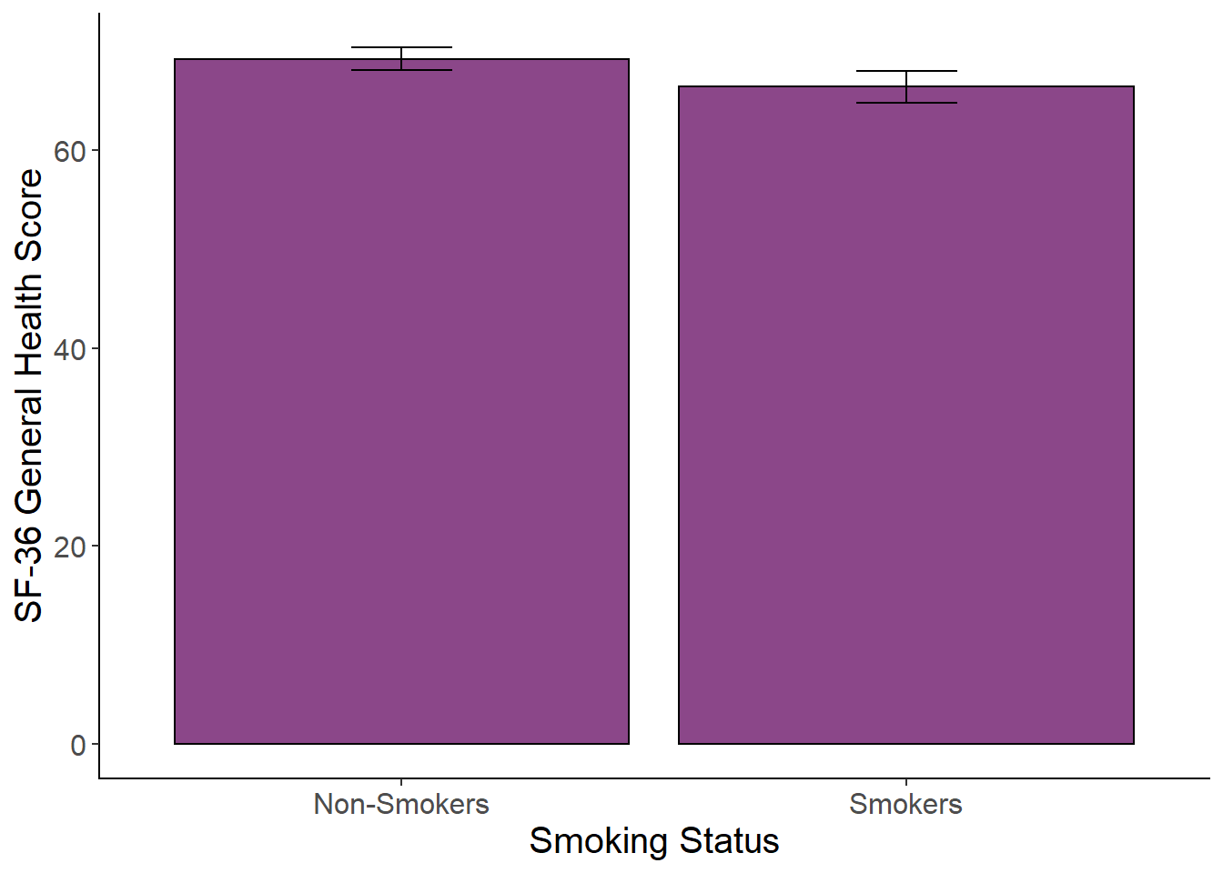
To examine whether there were mean differences between smokers and non-smokers on the SF-36 general health scale, an independent samples t-test was conducted. Levene’s test was not significant (p=.29). There was a significant difference between groups, t(1230)=2.84, p=.005, 95%CI[0.87, 4.75]. Non-smokers (M=69.23, SD = 16.32) had a higher general health score than smokers (M = 66.42, SD = 16.90).
Plotting the Means with SE
Create a plot of the means with standard error bars using the code below. The cleanup code at the beginning is used to remove the gray background and set the axis line colors to black. The rest of the code is the mean plot. In the code below,cases with missing data have been filtered out before running the plot. Try it without filtering out the missing data so see what happens.
#cleanup code (run once per R session)
cleanup = theme(panel.grid.major = element_blank(),
                panel.grid.minor = element_blank(),
                panel.background = element_blank(),
                axis.line.x = element_line(color = "black"),
                axis.line.y = element_line(color = "black"),
                legend.key = element_rect(fill = "white"),
                text = element_text(size = 15))

genhealth_plot <-smoking_noout %>%
  dplyr::filter(!is.na(smoker)) %>%
  ggplot(aes(x = smoker , y = general_health)) +
  stat_summary(fun.y = mean,
               geom = "bar",
               fill = "orchid4",
               color = "Black") +
  stat_summary(fun.data = mean_cl_normal,
               geom = "errorbar",
               width = .2,
               position = "dodge")  +
  xlab("Smoking Status") +
  ylab("SF-36 General Health Score") +
  scale_x_discrete(labels = c("Non-Smokers","Smokers")) +
  cleanup

genhealth_plot
Paired Samples T-Test
In repeated measures designs, each participant contributes scores to each condition. To compare 2 means in a repeated measures design, use a paired samples t-test (sometimes called a dependent samples t-test).
A study was conducted to see if completing a Sudoku puzzle every day for 2 weeks improved cognitive functioning in a sample of elderly adults (age 65+). A researcher collected data regarding cognitive performance for 20 elderly adults on a task before (T1) and after (T2) the two week intervention. Use a paired samples t-test to determine if cognitive performance improved from T1 to T2.
You can download the data for this exercise here: Download CogStudy Dataset
- What is the problem with the research design used in this study? How would you improve the study design?
Let’s load the dataset:
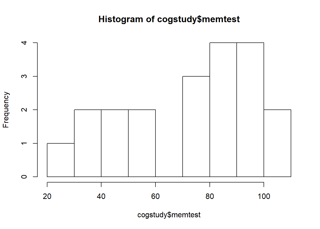
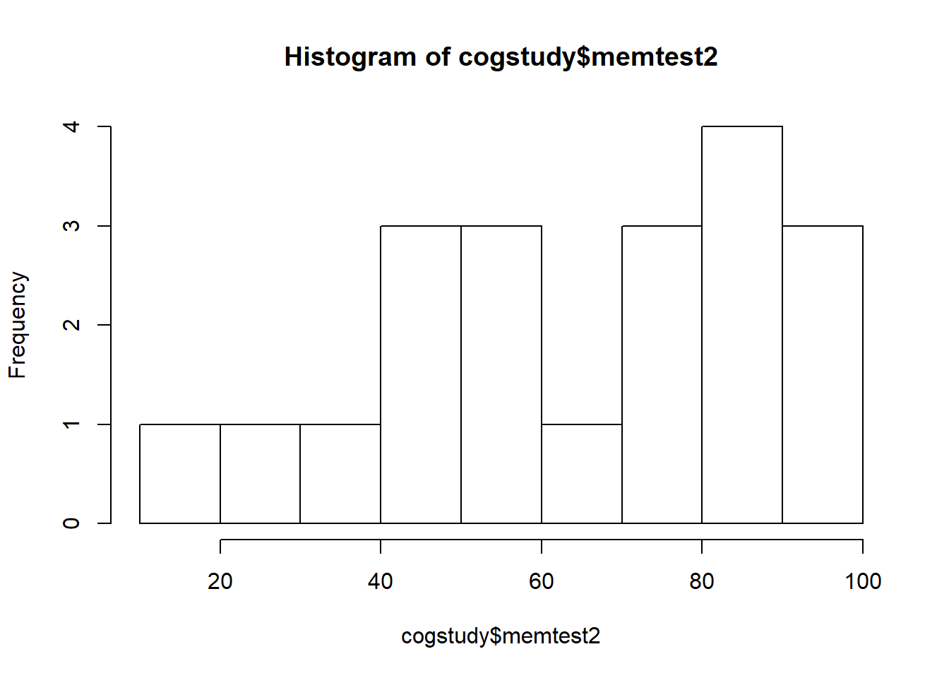
The two variables were are interested in are memtest (T1 scores) and memtest2 (T2 scores). The range of scores on the memory test should be betweeb 20-120. Check the dataset for accuracy, and then create a histogram for each set of scores.
#summary statistics
summary(cogstudy$memtest)
##    Min. 1st Qu.  Median    Mean 3rd Qu.    Max.
##   29.64   51.49   80.11   72.43   94.16  109.74
summary(cogstudy$memtest2)
##    Min. 1st Qu.  Median    Mean 3rd Qu.    Max.
##   17.94   41.76   69.56   64.44   86.87   99.28
#histograms
hist(cogstudy$memtest)
hist(cogstudy$memtest2)
Checking Assumptions
Next, we should check assumptions. Homogeneity of variance does not apply for dependent t-tests. The normality assumptions applies to the distribution of the difference scores. Let’s create a variable that represents the difference between memtest and memtest2 and then create a histogram of the difference scores.
#create difference scores
cogstudy$diff <- cogstudy$memtest - cogstudy$memtest2

#histogram of difference scores
hist(cogstudy$diff, breaks = 20)

It doesn’t look great. We should probably consider running this as a non-parametric test. But t-tests are pretty robust so let’s proceed with a parametric t-test anyway.
Running the paired samples T-Test
There are two ways we could run the test, both below. In the first example, the two variables are listed first separated by a , (and using the $ to indicate the dataset and variable name), and then the line paired=TRUE to account for the dependency in the data.
In the second example, we are running the t-test on the difference scores of the two variables, which is equivalent to a one-sample t-test.
t.test(cogstudy$memtest, cogstudy$memtest2, paired=TRUE)
##
## 	Paired t-test
##
## data:  cogstudy$memtest and cogstudy$memtest2
## t = 1.81, df = 19, p-value = 0.08615
## alternative hypothesis: true difference in means is not equal to 0
## 95 percent confidence interval:
##  -1.248393 17.213393
## sample estimates:
## mean of the differences
##                  7.9825
#paired samples t-test using same formula structure as the independent t-test
t.test(~(memtest-memtest2), data=cogstudy)
##
## 	One Sample t-test
##
## data:  (memtest - memtest2)
## t = 1.81, df = 19, p-value = 0.08615
## alternative hypothesis: true mean is not equal to 0
## 95 percent confidence interval:
##  -1.248393 17.213393
## sample estimates:
## mean of x
##    7.9825
- Write up the results of the paired samples t-test in APA format.
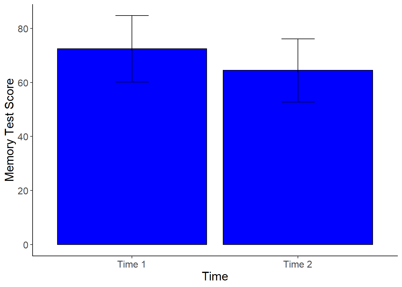
Plotting the Means: Dependent Samples T-Test
To plot the means for the dependent t-test in this example, we will need to restructure the data. Our data is currently in wide format where each participant gets one row, and all of the repeated measurements are in separate columns. We need the data to be in “long” format to create a bar graph. With long format data, each observation/repeated measurement gets it own line, so that each participant has multiple rows of data (equal to the number of measurment occasions). We can use the gather function from dplyr to do the restructuring. After restructuring, we will need to factor the new grouping variable that we created. Then we can create the plot using ggplot2. I’ve done this in two steps below so you can see how the restructuring works before you factor the new variable (you could do all of this in one code chunk with the %>%).
cogstudy_res <- cogstudy %>%
  gather(key = "Time", value = "Score", memtest:memtest2)

cogstudy_res <- cogstudy_res %>%
  mutate(Time = factor(Time,
                       levels = c("memtest", "memtest2"),
                       labels = c("Time 1", "Time 2")))


cogstudy_plot <-cogstudy_res %>%
  ggplot(aes(x = Time , y = Score)) +
  stat_summary(fun.y = mean,
               geom = "bar",
               fill = "blue",
               color = "Black") +
  stat_summary(fun.data = mean_cl_normal,
               geom = "errorbar",
               width = .2,
               position = "dodge")  +
  xlab("Time") +
  ylab("Memory Test Score") +
  cleanup

cogstudy_plot
Non-Parametric T-Tests
When you have a small sample (n<30), when your data violate the assumptions of a parametric tests, when the data is very skewed, or your data are ordinal, non-parametric tests can be used instead of parametric tests. With a non-parametric t-test, the data are ranked and the analysis is performed on the ranked data. When reporting the results of a non-parametric test, you should report the median, not the mean.
- Discussion question: Why should you report the median instead of a mean for non-parametric tests?
For this example, let’s make some data! We will compare two groups of 5 participants each on an outcome variable. After creating the data, calculate the median by group and create histograms.
group <- c(1,1,1,1,1,2,2,2,2,2)
outcome <- c(3,1,3,4,2,5,4,6,5,6)
Non-parametric T-Test for Independent Groups: Mann Whitney U
The non-paramteric version of the independent samplest t-test is the Mann Whitney U test.
wilcox.test(outcome~group)
## Warning in wilcox.test.default(x = c(3, 1, 3, 4, 2), y = c(5, 4, 6, 5, 6: cannot
## compute exact p-value with ties
##
## 	Wilcoxon rank sum test with continuity correction
##
## data:  outcome by group
## W = 0.5, p-value = 0.01502
## alternative hypothesis: true location shift is not equal to 0
How do we get a Mann Whitney U test from a function called wilcox? There is another non-parametric independent samples t-test that is equivalent to the MW-U called the Wilcoxon Rank Sum Test. And just to make things more confusing–the non-parametric version of the paired samples t-test is called the Wilcoxon Signed Rank Test.
Non-parametric T-Test for Dependent Groups: Wilcoxon Signed Rank Test
In the paired-samples t-test we did earlier, we only had 20 participants and the distribution was skewed. Let’s run the non-parametric test on the data and see if we get the similar results.
wilcox.test(cogstudy$memtest,cogstudy$memtest2, paired=TRUE)
##
## 	Wilcoxon signed rank test
##
## data:  cogstudy$memtest and cogstudy$memtest2
## V = 147, p-value = 0.1231
## alternative hypothesis: true location shift is not equal to 0