Analysis of Covariance (ANCOVA)
Through the first four weeks of this course, we have learned how to run correlations, simple regression models, simultaneous and hierarchical models with continuous variables, and have learned how to perform regression models with categorical predictors (analogous to ANOVA). This week, we will examine how to run an ANCOVA model–an analysis of covariance. ANCOVA can be used when you want to compare groups (categorical variable), but also want to control for the effects of a covariate (hence the “covariance” component of Analysis of covariance).
We will return to the neurological FIM dataset we have used in the past. You are a manager of rehabilitation services at a large healthcare system with several in-patient rehabilitation facilities. Your team has initiated a clinical trial to examine the effect of mode of treatment delivery on FIM outcomes. Patients receive one of three different modes of treatment delivery: group and individual therapy per day, individual therapy twice a day, or group therapy twice a day. One of your main research questions is the following: Do discharge FIM scores differ across the 3 treatment groups? The usual mode of delivery is individual therapy twice per day. You wonder if the other modes of delivery would get different results. You believe that the number of therapy sessions might have an influence on the change in FIM score.
- What is the IV? What is the DV? What are the TWO covariates you should include in the model?
We will start by loading and cleaning the dataset. We will need to factor the treatment variable, and then run some basic descriptive statistics to get a feel for what is going on with the data.
#loading the dataset
neuroFIM <- read_sav("neurological_FIM.sav")

#factoring the treatment variable
neuroFIM <- neuroFIM %>%
  mutate(treatment = as_factor(treatment))


#descriptives and boxplots
favstats(admfim~treatment, data=neuroFIM)
##                                       treatment min Q1 median Q3 max     mean
## 1 group therapy and individual therapy each day  18 57   68.5 79 123 68.00000
## 2              individual therapy twice per day  18 50   62.0 73 109 61.11020
## 3                   group therapy twice per day  18 42   53.5 70 100 55.14407
##         sd   n missing
## 1 16.46093 240       0
## 2 17.19107 245       0
## 3 18.17001 236       0
favstats(total_sessions~treatment, data=neuroFIM)
##                                       treatment min Q1 median Q3 max     mean
## 1 group therapy and individual therapy each day   0 12     17 23 157 20.81250
## 2              individual therapy twice per day   2 11     18 26 154 22.28980
## 3                   group therapy twice per day   1 12     18 27 107 22.12712
##         sd   n missing
## 1 18.39326 240       0
## 2 18.57444 245       0
## 3 16.79136 236       0
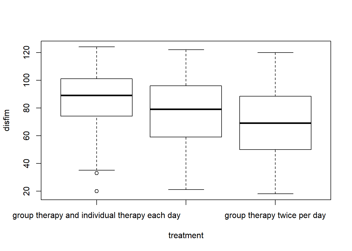
boxplot(disfim~treatment, data=neuroFIM)
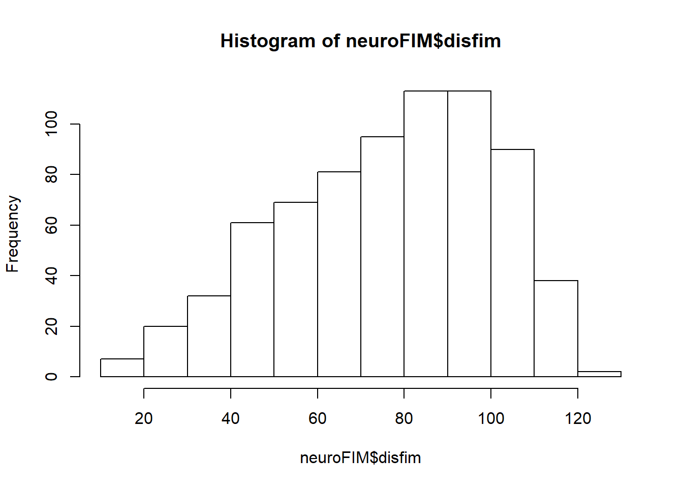
hist(neuroFIM$disfim)
Assumptions of ANCOVA
Correlations Between the Covariates
We have two covariates so we should check the correlation between them to make sure that it is not too high. We will also include the dependent variable to make sure that we have a correlation between the covariates and the DV.
neuroFIM %>%
  dplyr::select(admfim, disfim, total_sessions) %>%
  as.matrix() %>%
  rcorr(type="pearson")
##                admfim disfim total_sessions
## admfim           1.00   0.81          -0.19
## disfim           0.81   1.00           0.00
## total_sessions  -0.19   0.00           1.00
##
## n= 721
##
##
## P
##                admfim disfim total_sessions
## admfim                0.0000 0.0000
## disfim         0.0000        0.9651
## total_sessions 0.0000 0.9651
As you might expect, the admission and discharge scores are highly correlated. All other correlations are small. Interestingly, the total number of therapy sessions is not correlated with the outcome variable. Based on these results, it looks like we could just run the ANOVA model without the covariate included. In fact, running the ANCOVA with a covariate that is not correlated with the outcome can reduce statistical power. But we should investigate this a little further before we make any decisions. Let’s take a look at a scatterplot of the relationship between discharge FIM scores and the covariate, number of therapy sessions.
library(car)
scatterplot(disfim~total_sessions, data=neuroFIM, smooth=FALSE, ellipse=FALSE)
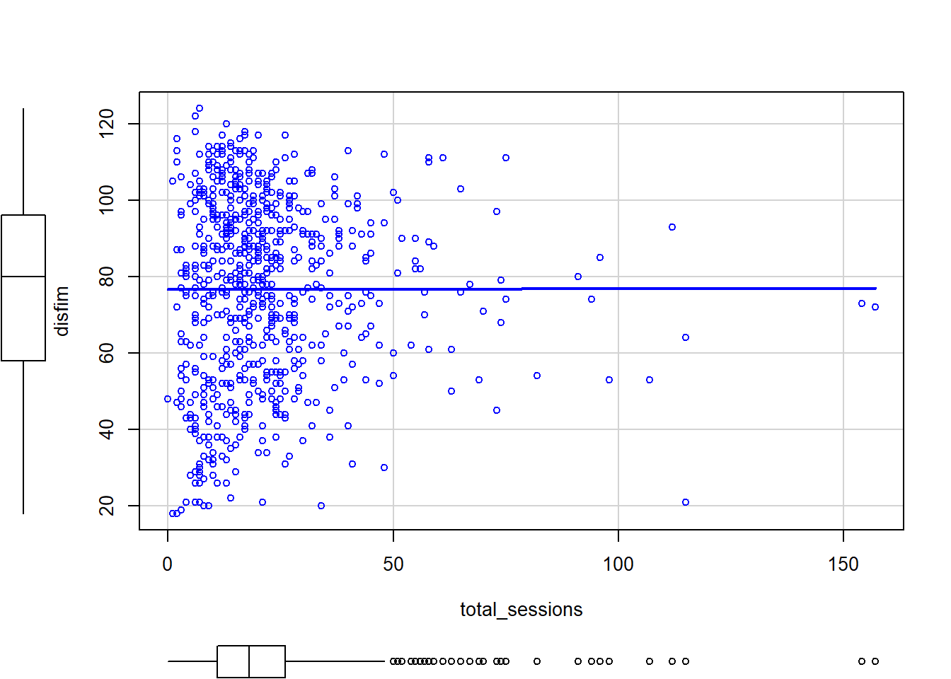
From this scatterplot, it looks like there may be some outliers. We can run regression diagnostics later to see if there are extreme/influential cases that need to be removed. Let’s also look at this scatterplot with the treatment group included.
scatterplot(disfim~total_sessions | treatment, data=neuroFIM, smooth=FALSE, ellipse=FALSE, col=c("black", "blue", "red"))
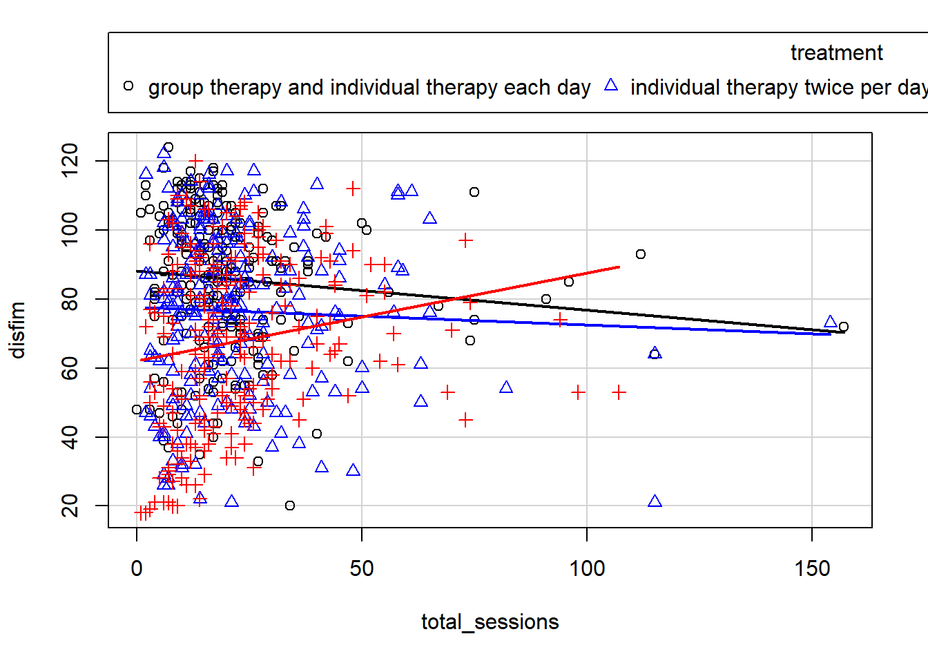
Here we can see that the relationship is positive for the Group Therapy treatment, and slightly negative for the other two treatment types. However, we also have those two outlier cases which may be having an impact on the correlation. For now, we will proceed with the ANCOVA analysis and run regression diagnostics to see if we need to remove those cases.
Homogeneity of Variance
Before we get to regression diagnostics, we shoulde take a look at the assumption of homogeneity of variance. Because we have a between subjects design, we need to be confirm that we have homogeneity of variance across the levels of our independent variable. Use the LevenesTest function from the car package to test this assumption.
library(car)
leveneTest(disfim~treatment, data=neuroFIM, center=mean)
## Levene's Test for Homogeneity of Variance (center = mean)
##        Df F value    Pr(>F)
## group   2  7.1489 0.0008429 ***
##       718
## ---
## Signif. codes:  0 '***' 0.001 '**' 0.01 '*' 0.05 '.' 0.1 ' ' 1
Levene’s Test indicates that we have violated the assumption of homogeneity of variance. HOWEVER–Levene’s test is sensitive to sample size, and visual inspection of the data (boxpots, variance) demonstrates that we probably don’t need to be concerned about violating homogeneity of variance. So we will happily proceed with our analyses.
- If you were doing a RMANCOVA (repeated measures ANCOVA), what assumption(s) would you need to check?
Homogeneity of Regression Slopes
To test homogeneity of the regression slopes, we can include an interaction term between the two variables when we run the regression model. If the interaction is not significant, then we have independence of the covariate and IV. We can then re-run the regression model and drop the interaction term.
mod1 <- lm(disfim ~ admfim*treatment + treatment*total_sessions, data=neuroFIM)
summary(mod1)
##
## Call:
## lm(formula = disfim ~ admfim * treatment + treatment * total_sessions,
##     data = neuroFIM)
##
## Residuals:
##     Min      1Q  Median      3Q     Max
## -70.049  -8.193  -1.320   7.738  54.438
##
## Coefficients:
##                                                            Estimate Std. Error
## (Intercept)                                               12.147762   4.252560
## admfim                                                     1.028642   0.054870
## treatmentindividual therapy twice per day                 -4.804192   5.569148
## treatmentgroup therapy twice per day                     -13.803197   5.211772
## total_sessions                                             0.174393   0.049106
## admfim:treatmentindividual therapy twice per day           0.039314   0.074745
## admfim:treatmentgroup therapy twice per day                0.116447   0.072657
## treatmentindividual therapy twice per day:total_sessions   0.002201   0.067956
## treatmentgroup therapy twice per day:total_sessions        0.107585   0.071186
##                                                          t value Pr(>|t|)
## (Intercept)                                                2.857 0.004407 **
## admfim                                                    18.747  < 2e-16 ***
## treatmentindividual therapy twice per day                 -0.863 0.388624
## treatmentgroup therapy twice per day                      -2.648 0.008265 **
## total_sessions                                             3.551 0.000408 ***
## admfim:treatmentindividual therapy twice per day           0.526 0.599068
## admfim:treatmentgroup therapy twice per day                1.603 0.109447
## treatmentindividual therapy twice per day:total_sessions   0.032 0.974171
## treatmentgroup therapy twice per day:total_sessions        1.511 0.131151
## ---
## Signif. codes:  0 '***' 0.001 '**' 0.01 '*' 0.05 '.' 0.1 ' ' 1
##
## Residual standard error: 13.26 on 712 degrees of freedom
## Multiple R-squared:  0.6951,	Adjusted R-squared:  0.6916
## F-statistic: 202.9 on 8 and 712 DF,  p-value: < 2.2e-16
Neither of the interaction terms are significant, so we appear to have homogeneity of the regression slopes.
Independence of the Covariate and IV
To test whether our covariates are related to the IV, we can use an ANOVA model with the covariate as the dependent variable and the IV as the predictor. Because we have two covariates, we should do this once for each covariate.
library(ez)
anova_mod1 <- ezANOVA(data=neuroFIM,
                      wid = PtID,
                      between = treatment,
                      dv = total_sessions,
                      type = 3,
                      detailed = TRUE)
print(anova_mod1)
## $ANOVA
##        Effect DFn DFd         SSn      SSd            F             p p<.05
## 1 (Intercept)   1 718 340783.0460 231297.2 1057.8695079 2.488376e-143     *
## 2   treatment   2 718    315.8696 231297.2    0.4902661  6.126682e-01
##           ges
## 1 0.595691014
## 2 0.001363781
##
## $`Levene's Test for Homogeneity of Variance`
##   DFn DFd      SSn      SSd        F         p p<.05
## 1   2 718 370.3674 156777.3 0.848094 0.4286589
anova_mod2 <- ezANOVA(data=neuroFIM,
                      wid = PtID,
                      between = treatment,
                      dv = admfim,
                      type = 3,
                      detailed = TRUE)
print(anova_mod2)
## $ANOVA
##        Effect DFn DFd        SSn      SSd          F            p p<.05
## 1 (Intercept)   1 718 2719106.08 214455.1 9103.62087 0.000000e+00     *
## 2   treatment   2 718   19709.38 214455.1   32.99369 1.957576e-14     *
##          ges
## 1 0.92689598
## 2 0.08416893
##
## $`Levene's Test for Homogeneity of Variance`
##   DFn DFd      SSn      SSd        F          p p<.05
## 1   2 718 480.6125 74053.94 2.329922 0.09803864
Results of the ANOVAs demonstrate that total_sessions is not related to the treatment variable. However, there were significant differences between the treatment groups on admission scores. It is likely that the original study did not randomly assign participants to a treatment condition (or their attempt to randomly assign did not work). We stil want to include pre-treatment scores in our analysis, so we will proceed with the analysis. Alternatively, we could calculate a change score between pre- and post-treatment and use that as the dependent variable (change score analysis). However, if this was a true experimental design, controlling for T1 is the preferred analysis over change scores.
Running the ANCOVA Model
Now we can run the full ANCOVA model. To do so, we will use the lm function. I’m going to save this one to an object called “final_model” because we will use it to examine regression diagnostics
final_model <- lm(disfim ~ admfim + total_sessions + treatment, data = neuroFIM)
summary(final_model)
##
## Call:
## lm(formula = disfim ~ admfim + total_sessions + treatment, data = neuroFIM)
##
## Residuals:
##     Min      1Q  Median      3Q     Max
## -70.104  -8.451  -1.392   8.173  53.581
##
## Coefficients:
##                                           Estimate Std. Error t value Pr(>|t|)
## (Intercept)                                7.11561    2.33600   3.046 0.002404
## admfim                                     1.09068    0.02919  37.362  < 2e-16
## total_sessions                             0.21347    0.02811   7.594 9.69e-14
## treatmentindividual therapy twice per day -1.98290    1.22160  -1.623 0.104987
## treatmentgroup therapy twice per day      -4.25505    1.27188  -3.345 0.000864
##
## (Intercept)                               **
## admfim                                    ***
## total_sessions                            ***
## treatmentindividual therapy twice per day
## treatmentgroup therapy twice per day      ***
## ---
## Signif. codes:  0 '***' 0.001 '**' 0.01 '*' 0.05 '.' 0.1 ' ' 1
##
## Residual standard error: 13.27 on 716 degrees of freedom
## Multiple R-squared:  0.6928,	Adjusted R-squared:  0.6911
## F-statistic: 403.7 on 4 and 716 DF,  p-value: < 2.2e-16
summary.aov(final_model)
##                 Df Sum Sq Mean Sq  F value   Pr(>F)
## admfim           1 272157  272157 1544.636  < 2e-16 ***
## total_sessions   1  10422   10422   59.151 4.84e-14 ***
## treatment        2   1975     988    5.605  0.00384 **
## Residuals      716 126155     176
## ---
## Signif. codes:  0 '***' 0.001 '**' 0.01 '*' 0.05 '.' 0.1 ' ' 1
car::Anova(final_model, type = "III")
## Anova Table (Type III tests)
##
## Response: disfim
##                Sum Sq  Df   F value    Pr(>F)
## (Intercept)      1635   1    9.2785  0.002404 **
## admfim         245957   1 1395.9415 < 2.2e-16 ***
## total_sessions  10162   1   57.6731 9.687e-14 ***
## treatment        1975   2    5.6050  0.003843 **
## Residuals      126155 716
## ---
## Signif. codes:  0 '***' 0.001 '**' 0.01 '*' 0.05 '.' 0.1 ' ' 1
Remember we use an ANOVA model when we want to compare means across conditions, and an ANCOVA model when we want to compare means but adjust for a covariate. The above regression analysis tells us that our two covariates are statistically significant, and that the group therapy 2x/day condition is significantly different from the individual + group therapy condition. Remember that R uses the first group as the reference category, so we end up with two comparisons in the regression–individual therapy 2x/day versus Group+ Individual therapy, and group therapy 2x/day versus Group+ Individual therapy. But because individual therapy 2x/day is the usual standard of care, it makes more sense to use that as the reference group. The other benefit of re-running the model with a different reference group is that we will now have all possible mean comparisons available. There are a couple different ways we could change the reference group. For this example, we will use the relevel function, and then re-run the model.
neuroFIM <- neuroFIM %>%
  mutate(treatment = relevel(treatment, ref = 2))

final_model_releveled <- lm(disfim ~ admfim + total_sessions + treatment, data = neuroFIM)
summary(final_model_releveled)
##
## Call:
## lm(formula = disfim ~ admfim + total_sessions + treatment, data = neuroFIM)
##
## Residuals:
##     Min      1Q  Median      3Q     Max
## -70.104  -8.451  -1.392   8.173  53.581
##
## Coefficients:
##                                                        Estimate Std. Error
## (Intercept)                                             5.13271    2.17202
## admfim                                                  1.09068    0.02919
## total_sessions                                          0.21347    0.02811
## treatmentgroup therapy and individual therapy each day  1.98290    1.22160
## treatmentgroup therapy twice per day                   -2.27214    1.22328
##                                                        t value Pr(>|t|)
## (Intercept)                                              2.363   0.0184 *
## admfim                                                  37.362  < 2e-16 ***
## total_sessions                                           7.594 9.69e-14 ***
## treatmentgroup therapy and individual therapy each day   1.623   0.1050
## treatmentgroup therapy twice per day                    -1.857   0.0637 .
## ---
## Signif. codes:  0 '***' 0.001 '**' 0.01 '*' 0.05 '.' 0.1 ' ' 1
##
## Residual standard error: 13.27 on 716 degrees of freedom
## Multiple R-squared:  0.6928,	Adjusted R-squared:  0.6911
## F-statistic: 403.7 on 4 and 716 DF,  p-value: < 2.2e-16
Note that the overall model statistics did not change (F, \(R^2\)). However, the intercept changed and we now have a coefficient for individual therapy 2x/day versus group therapy 2x/day.
- Why did the intercept change when re-running the model with a difference reference group?
Regression Diagnostics
To make things a little easier on ourselves for this example, let’s create a smaller dataset that only contains the variables we are using in the analysis. Then, we will check regression diagnostics using this smaller dataset. Remember that categorical variables need to be excluded to accuarately calculate Mahalanobis distances.
#creating a smaller dataset
neuroFIM_short <- neuroFIM %>%
  dplyr::select(admfim,disfim,total_sessions,treatment)

#mahalanobis distance
mahal = mahalanobis(neuroFIM_short[,-4],
                    colMeans(neuroFIM_short[,-4]),
                    cov(neuroFIM_short[,-4]))

mahal_cutoff = qchisq(1-.001, ncol(neuroFIM_short[,-4]))
badmahal = as.numeric(mahal > mahal_cutoff)
table(badmahal)
## badmahal
##   0   1
## 706  15
#leverage
k = 4
leverage = hatvalues(final_model)
cutleverage = (2*k+2) / nrow(neuroFIM_short)
badleverage = as.numeric(leverage > cutleverage)
table(badleverage)
## badleverage
##   0   1
## 694  27
#cooks
cooks = cooks.distance(final_model)
cutcooks = 4 / (nrow(neuroFIM_short) - k - 1)
cutcooks ##get the cut off
## [1] 0.005586592
badcooks = as.numeric(cooks > cutcooks)
table(badcooks)
## badcooks
##   0   1
## 682  39
##add them up!
totalout = badmahal + badleverage + badcooks
table(totalout)
## totalout
##   0   1   2   3
## 668  34  10   9
neuroFIM_noout <- subset(neuroFIM_short, totalout <2)
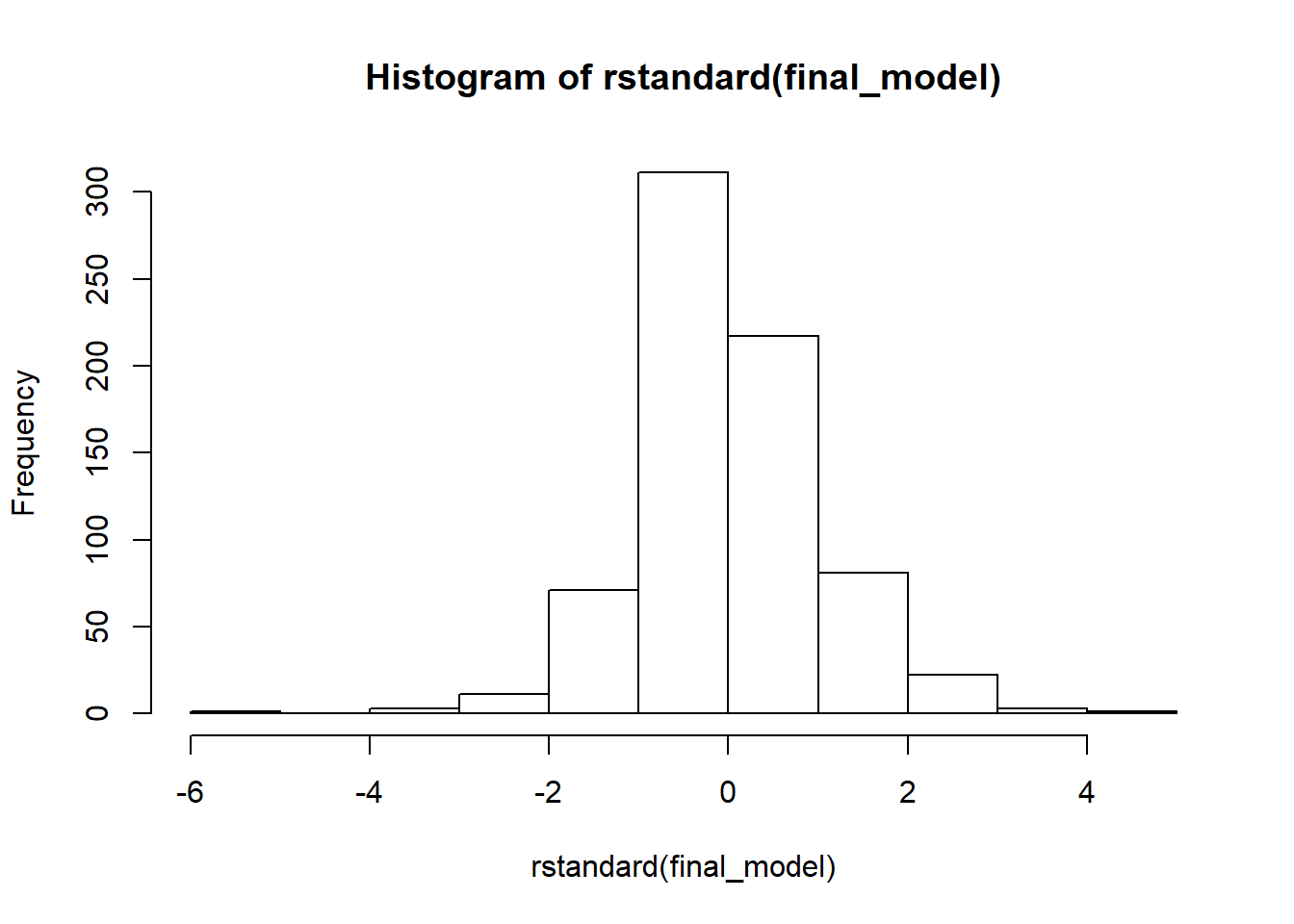
#histograms of the residuals
hist(rstandard(final_model))
hist(rstudent(final_model))

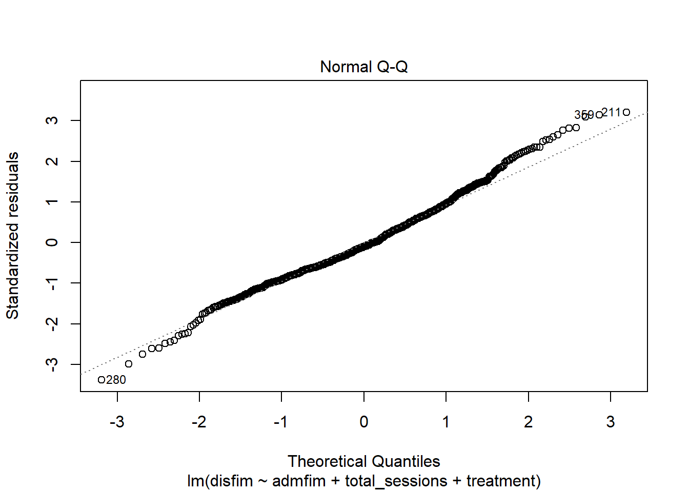
qqPlot(final_model)
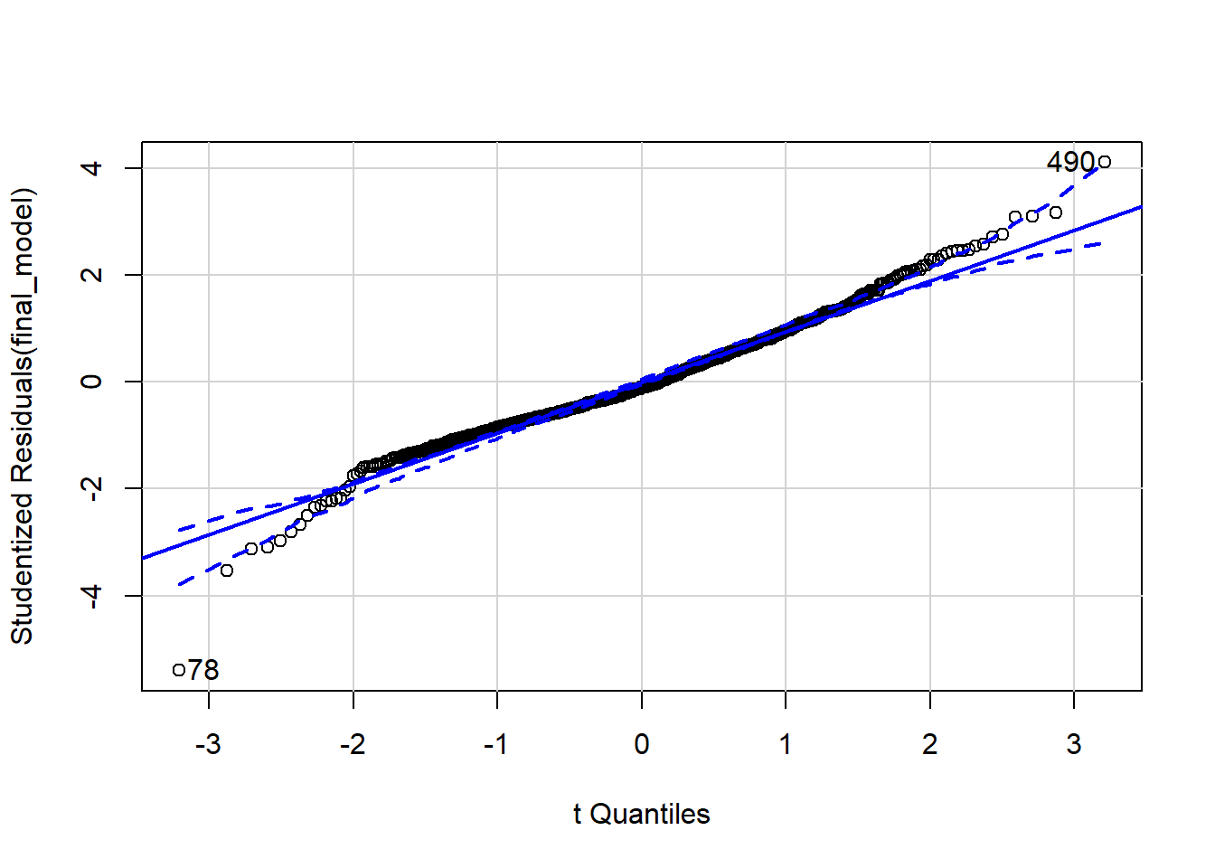
## [1] 78 490
#re-running the model with the outliers removed
neuroFIM_noout <- subset(neuroFIM_short, mahal < mahal_cutoff) ##exclude outliers

final_model_noout <- lm(disfim ~ admfim + total_sessions + treatment, data = neuroFIM_noout)
summary(final_model_noout)
##
## Call:
## lm(formula = disfim ~ admfim + total_sessions + treatment, data = neuroFIM_noout)
##
## Residuals:
##     Min      1Q  Median      3Q     Max
## -41.381  -7.930  -1.204   7.537  39.251
##
## Coefficients:
##                                                        Estimate Std. Error
## (Intercept)                                             1.22863    2.08049
## admfim                                                  1.11911    0.02721
## total_sessions                                          0.35646    0.03507
## treatmentgroup therapy and individual therapy each day  1.39665    1.14290
## treatmentgroup therapy twice per day                   -2.92419    1.14340
##                                                        t value Pr(>|t|)
## (Intercept)                                              0.591   0.5550
## admfim                                                  41.122   <2e-16 ***
## total_sessions                                          10.164   <2e-16 ***
## treatmentgroup therapy and individual therapy each day   1.222   0.2221
## treatmentgroup therapy twice per day                    -2.557   0.0108 *
## ---
## Signif. codes:  0 '***' 0.001 '**' 0.01 '*' 0.05 '.' 0.1 ' ' 1
##
## Residual standard error: 12.27 on 701 degrees of freedom
## Multiple R-squared:  0.7363,	Adjusted R-squared:  0.7348
## F-statistic: 489.4 on 4 and 701 DF,  p-value: < 2.2e-16
outlierTest(final_model_noout)
## No Studentized residuals with Bonferroni p < 0.05
## Largest |rstudent|:
##     rstudent unadjusted p-value Bonferroni p
## 280 -3.40783          0.0006923      0.48876
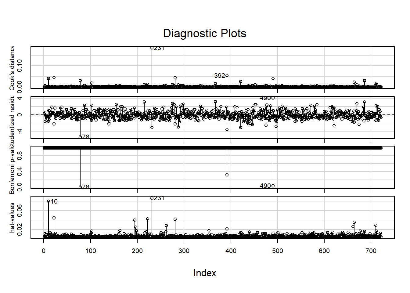
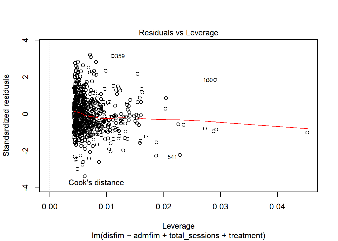
influenceIndexPlot(final_model)
vif(final_model)
##                    GVIF Df GVIF^(1/(2*Df))
## admfim         1.132556  1        1.064216
## total_sessions 1.038647  1        1.019140
## treatment      1.093112  2        1.022507
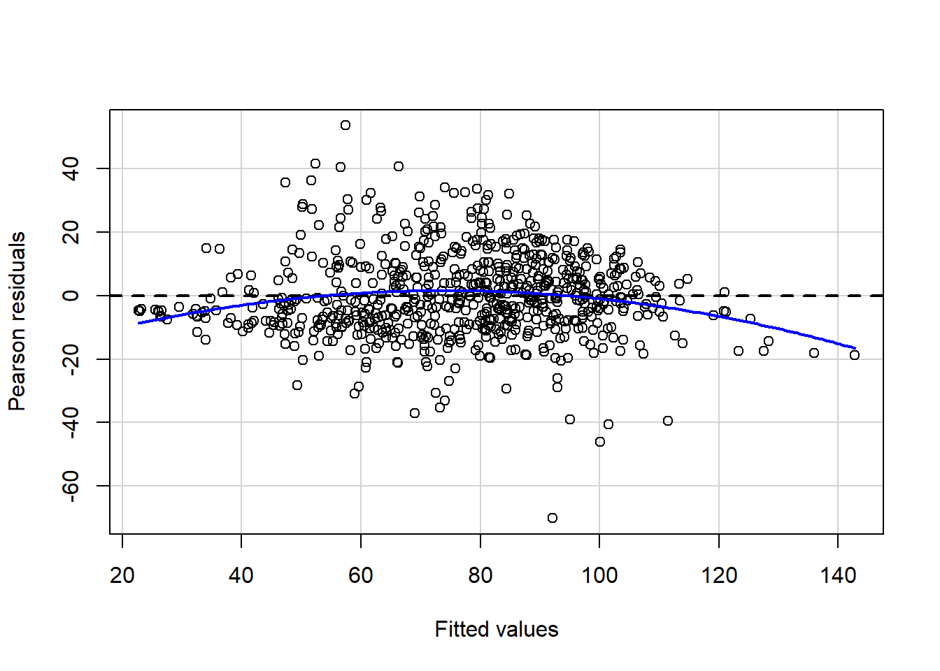
ncvTest(final_model)
## Non-constant Variance Score Test
## Variance formula: ~ fitted.values
## Chisquare = 0.569546, Df = 1, p = 0.45044
residualPlot(final_model)
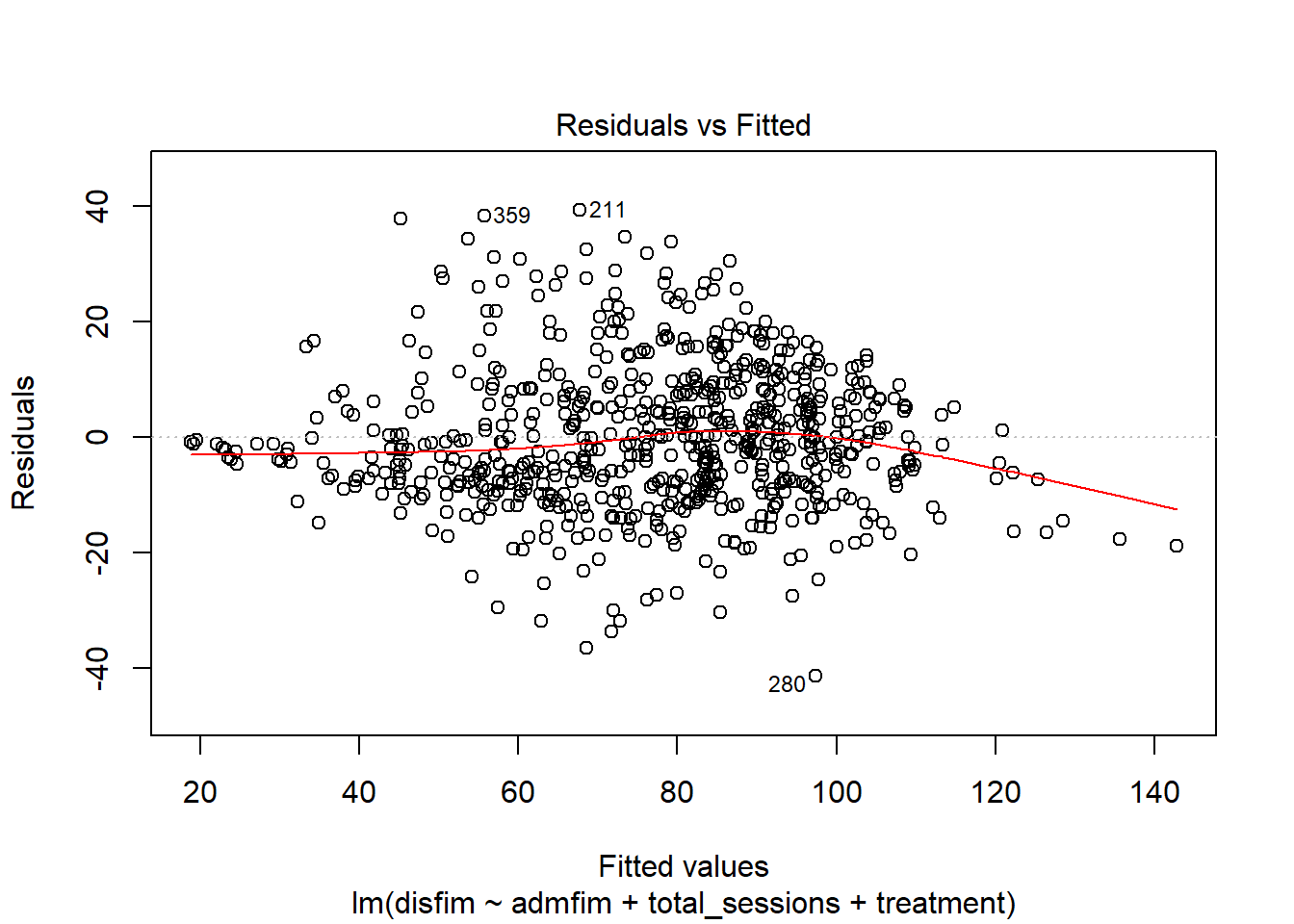
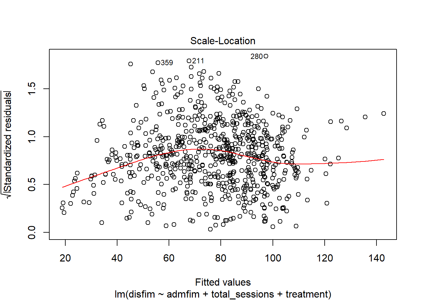
plot(final_model_noout)
compareCoefs(final_model_releveled, final_model_noout)
## Calls:
## 1: lm(formula = disfim ~ admfim + total_sessions + treatment, data =
##   neuroFIM)
## 2: lm(formula = disfim ~ admfim + total_sessions + treatment, data =
##   neuroFIM_noout)
##
##                                                        Model 1 Model 2
## (Intercept)                                               5.13    1.23
## SE                                                        2.17    2.08
##
## admfim                                                  1.0907  1.1191
## SE                                                      0.0292  0.0272
##
## total_sessions                                          0.2135  0.3565
## SE                                                      0.0281  0.0351
##
## treatmentgroup therapy and individual therapy each day    1.98    1.40
## SE                                                        1.22    1.14
##
## treatmentgroup therapy twice per day                     -2.27   -2.92
## SE                                                        1.22    1.14
##
Graphing the Means
Because we are interested in mean comparisons, it would be helpful to graph the adjusted means and corresponding confidence intervals. We can use the emmeans package we used last semester to get the adjusted means for an ANCOVA model. We can even request the contrasts! These numbers should correspond to what we get in our regresssion model (double check!)
library(emmeans)
emmeans(final_model_noout,pairwise ~treatment)
## $emmeans
##  treatment                                     emmean    SE  df lower.CL
##  individual therapy twice per day                77.4 0.796 701     75.9
##  group therapy and individual therapy each day   78.8 0.818 701     77.2
##  group therapy twice per day                     74.5 0.823 701     72.9
##  upper.CL
##      79.0
##      80.4
##      76.1
##
## Confidence level used: 0.95
##
## $contrasts
##  contrast
##  individual therapy twice per day - group therapy and individual therapy each day
##  individual therapy twice per day - group therapy twice per day
##  group therapy and individual therapy each day - group therapy twice per day
##  estimate   SE  df t.ratio p.value
##     -1.40 1.14 701 -1.222  0.4405
##      2.92 1.14 701  2.557  0.0289
##      4.32 1.19 701  3.642  0.0008
##
## P value adjustment: tukey method for comparing a family of 3 estimates
favstats(disfim~treatment, data=neuroFIM)
##                                       treatment min Q1 median     Q3 max
## 1              individual therapy twice per day  21 59     79  96.00 122
## 2 group therapy and individual therapy each day  20 74     89 101.00 124
## 3                   group therapy twice per day  18 50     69  88.25 120
##       mean       sd   n missing
## 1 76.54286 23.59501 245       0
## 2 85.72500 20.17889 240       0
## 3 67.72881 24.32079 236       0
Another package that we could use to get and graph the means and standard errors is the effects package. The effects package combines nicely with ggplot2 to create a graph of the means.
library(effects)
#getting the means
effect_treatment = effect("treatment",final_model_noout)
effect_treatment <- as.data.frame(effect_treatment)
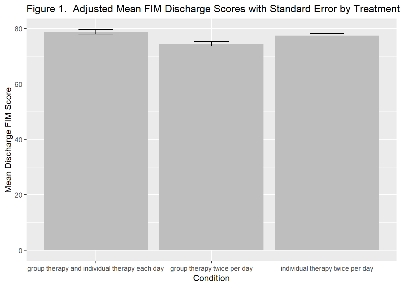
#plotting the means
plot_treatment <- ggplot(effect_treatment, aes(x=treatment, y=fit)) +
geom_bar(stat='identity', fill = "grey") +
geom_errorbar(aes(ymin=fit-se, ymax=fit+se,), width=.3,col="black") +
labs(x = "Condition", y = "Mean Discharge FIM Score") +
ggtitle("Figure 1. Adjusted Mean FIM Discharge Scores with Standard Error by Treatment Type")
plot_treatment

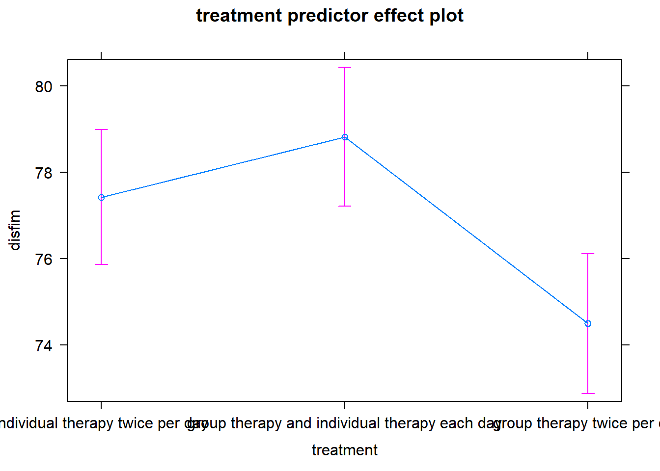
The effects package can also be combined with the plot function to create a line graph of the means.
#effect plot for treatment
plot(predictorEffect("treatment", final_model_noout))
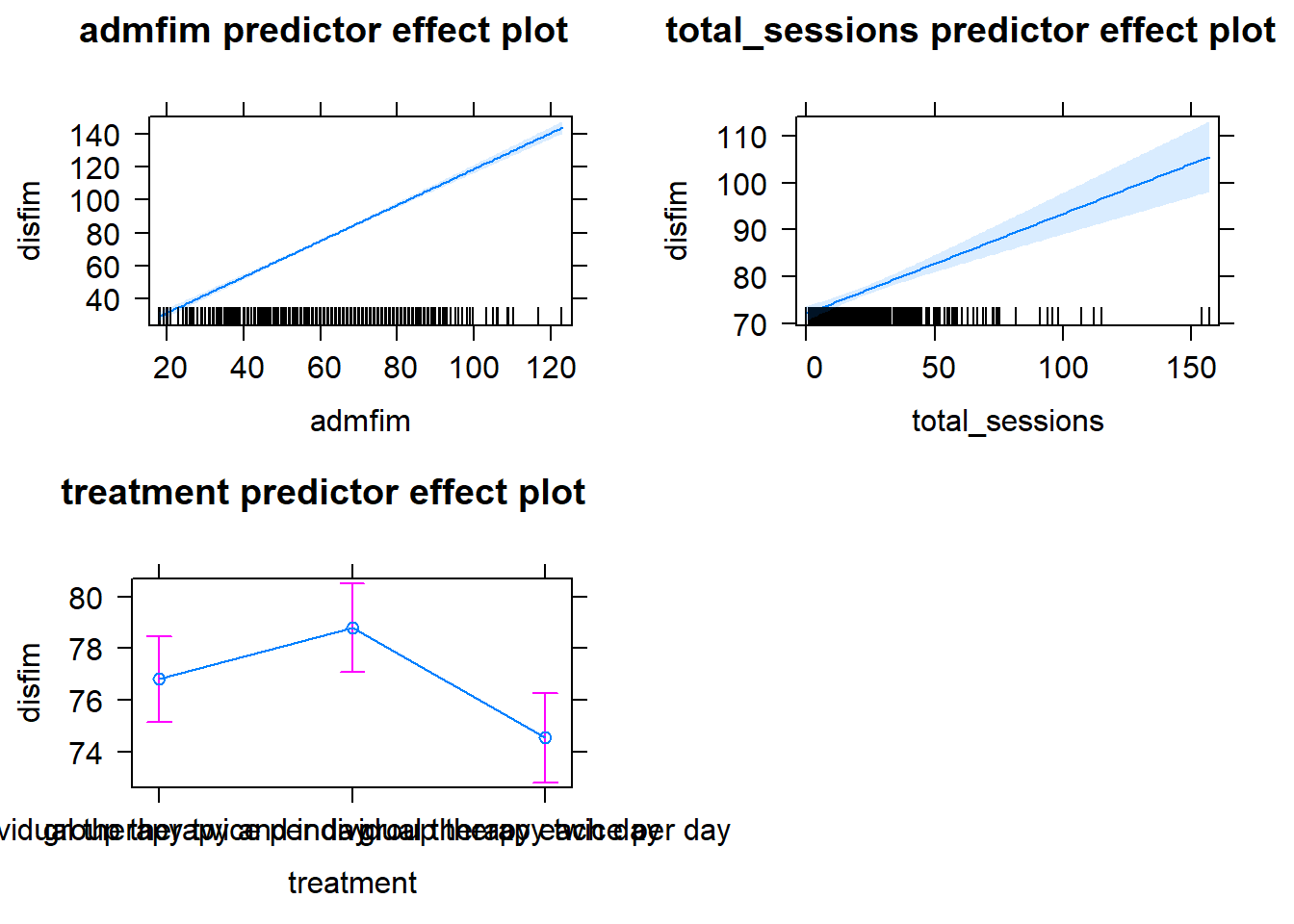
#all of the effect plots for the predictors in the model
plot(predictorEffects(final_model_releveled))
Writing it up!
To determine if other modes of therapy delivery are more (or less) effective than usual care (individual therapy 2x/day) we used an ANCOVA model, adjusting for admission scores and the number of therapy sessions. The overall model was statisticall significant, F(4,716) = 403.7, R^2 = .693, p<.001. Table 1 contains the results of the analysis. There were no significant differences between the usual care condition (individual therapy 2x/day) and the other two forms of therapy–group therapy 2x/day (p = .064) or individual and group therapy (p = .105). Figure 1 contains a graph of the means for each condition with their standard errors.
stargazer(final_model_releveled,
          type= "html",
          title = "Table 1.  ANCOVA Model Predicting FIM Discharge Scores",
          intercept.bottom = FALSE,
          covariate.labels = c("Intercept", "Admission FIM", "Total Therapy Sessions", "Usual care v. Group + Individual Therapy", "Usual Care v. Group Therapy 2x/day"),
          dep.var.labels = "Discharge FIM",
          dep.var.caption = "",
          single.row = TRUE,
          column.labels = "<i>b(SE)</i>")
| Discharge FIM | |
| b(SE) | |
| Intercept | 5.133** (2.172) |
| Admission FIM | 1.091*** (0.029) |
| Total Therapy Sessions | 0.213*** (0.028) |
| Usual care v. Group + Individual Therapy | 1.983 (1.222) |
| Usual Care v. Group Therapy 2x/day | -2.272* (1.223) |
| Observations | 721 |
| R2 | 0.693 |
| Adjusted R2 | 0.691 |
| Residual Std. Error | 13.274 (df = 716) |
| F Statistic | 403.749*** (df = 4; 716) |
| Note: | *p<0.1; **p<0.05; ***p<0.01 |