Categorical Predictors
This week we will focus on running and interpreting regression analyses with categorical predictors. We will use the NELS dataset referenced in the Keith book. The questions we are interested in answering are: Does family structure affect adolescents’ use of dangerous and illegal substances? Are adolescents from intact families less or more likely to use alcohol, tobacco, and other drugs? (Keith, page 120).
NELS <- read_sav("NELS n=1000.sav")
Data Preparation
Before we dive into the regression analysis, we first need to create the variables that we need for the analysis. The NELS dataset as a variable called FamComp that has 6 levels:
1 = Mother & father
2 = Mother and male guardian
3 = Father and female guardian
4 = Other two adult families
5 = Adult female only
6 = Adult male only
We are interested in comparing three groups of adolescents: those who live with 2 parents, those who live with one parent and one guardian, and those who live with a single parent. We will need to do some recoding/collapsing before we are ready to analyze this variable. To create a famstruc variable, we will leave group 1 alone, collapse groups 2 and 3, delete group 4, and collapse groups 5 and 6. All other groups/levels will be dropped from the variable. We will use the forcats package to help recode the variable into what we need.
NELS <- NELS %>%
  mutate(famcomp = as_factor(famcomp),
         famstruc = fct_collapse(famcomp, "Two-parent family" = c("MOTHER & FATHER"),
                                 "One parent, one guardian" = c("MOTHER & MALE GUARDN", "FEMALE GDN & FATHER"),
                                 "Single-parent family" = c("ADULT FEMALE ONLY", "ADULT MALE ONLY")),
         famstruc = factor(famstruc, levels = c("Two-parent family", "One parent, one guardian", "Single-parent family")))

#checking to make sure that the categories add up to what they should
fct_count(NELS$famcomp)
## # A tibble: 11 x 2
##    f                        n
##    <fct>                <int>
##  1 MOTHER & FATHER        677
##  2 MOTHER & MALE GUARDN   101
##  3 FEMALE GDN & FATHER     17
##  4 OTH 2 ADULT FAMILIES     8
##  5 ADULT FEMALE ONLY      156
##  6 ADULT MALE ONLY         21
##  7 MULTIPLE RESPONSE        0
##  8 REFUSAL                  0
##  9 MISSING                  0
## 10 LEGITIMATE SKIP          0
## 11 <NA>                    20
fct_count(NELS$famstruc)
## # A tibble: 4 x 2
##   f                            n
##   <fct>                    <int>
## 1 Two-parent family          677
## 2 One parent, one guardian   118
## 3 Single-parent family       177
## 4 <NA>                        28
There isn’t a general substance abuse variable in the NELS dataset, but there are several questions that we could combine to create a composite of substance abuse. Create a variable that is the mean of f1s77, f1s78a, and f1s80aa. These three variables represent lifetime total use of cigarettes, alcohol, and marijuana. These variables were measured on different scales, so we will need to standardized them before we create the composite variable.
#creating z-scores
NELS <- NELS %>%
  mutate(zf1s77 = scale(f1s77),
         zf1s78a = scale(f1s78a),
         zf1s80aa = scale(f1s80aa))

summary(NELS$zf1s77)
##        V1
##  Min.   :-0.3668
##  1st Qu.:-0.3668
##  Median :-0.3668
##  Mean   : 0.0000
##  3rd Qu.:-0.3668
##  Max.   : 5.1786
##  NA's   :96
#creating the substance abuse variable
NELS <- NELS %>%
  mutate(Substance = rowMeans(dplyr::select(NELS, zf1s77, zf1s78a, zf1s80aa)))

#descriptive statistics
favstats(~Substance, data=NELS)
##        min         Q1     median        Q3      max          mean        sd   n
##  -0.811183 -0.4874187 -0.1636545 0.2060405 3.349166 -0.0007963072 0.7720046 855
##  missing
##      145
ANOVA versus Regression with Categorical Predictors
As you might remember from last semester, if we have a categorical IV and a continuous DV, we can use an ANOVA to compare the means across groups. In this example, we have one categorical IV with 3 levels, and a continuous DV. So let’s run this as a one-way ANOVA and graph the means. ezANOVA has trouble with missing data so I am going to create a smaller dataset with just the variables we need first that contains only complete cases.
#examining the means and standard deviations by the famstructure variable
favstats(Substance ~ famstruc, data = NELS)
##                   famstruc       min         Q1       median        Q3      max
## 1        Two-parent family -0.811183 -0.4874187 -0.163654467 0.1601098 3.349166
## 2 One parent, one guardian -0.811183 -0.4874187 -0.001772328 0.5298047 2.979471
## 3     Single-parent family -0.811183 -0.4874187 -0.163654467 0.6414183 2.979471
##          mean        sd   n missing
## 1 -0.05845186 0.7262071 597      80
## 2  0.11956000 0.7615271  94      24
## 3  0.19184481 0.9361701 142      35
#creating dataset with no missing
NELS_short <- NELS %>%
  dplyr::select(stu_ids, famstruc, Substance) %>%
  na.omit()  #removes cases with missing data

#running the anova model
anova_model <- ezANOVA(data=NELS_short,
                       wid = stu_ids,
                       between=famstruc,
                       dv = Substance,
                       type = 3,
                       detailed= TRUE,
                       return_aov = TRUE)
print(anova_model)
## $ANOVA
##        Effect DFn DFd      SSn      SSd        F            p p<.05        ges
## 1 (Intercept)   1 830 3.305773 491.8238 5.578809 0.0184090634     * 0.00667658
## 2    famstruc   2 830 8.594215 491.8238 7.251782 0.0007547294     * 0.01717407
##
## $`Levene's Test for Homogeneity of Variance`
##   DFn DFd      SSn      SSd        F            p p<.05
## 1   2 830 5.092453 282.1811 7.489404 0.0005975776     *
##
## $aov
## Call:
##    aov(formula = formula(aov_formula), data = data)
##
## Terms:
##                 famstruc Residuals
## Sum of Squares    8.5942  491.8238
## Deg. of Freedom        2       830
##
## Residual standard error: 0.7697784
## Estimated effects may be unbalanced
The above results correspond to the SPSS results presented in Keith on page 120-121. The overall ANOVA is statistically significant, F(2,830) = 7.25, p <.001. Let’s now graph the means and examine post-hoc mean comparisons to see which groups are significantly different from one another.
cleanup = theme(panel.grid.major = element_blank(),
panel.grid.minor = element_blank(),
panel.background = element_blank(),
axis.line.x = element_line(color = "black"),
axis.line.y = element_line(color = "black"),
legend.key = element_rect(fill = "white"),
text = element_text(size = 15))
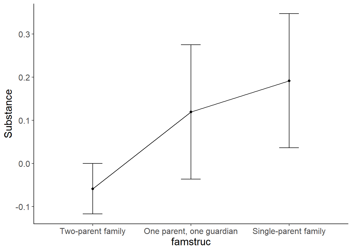
mean_plot <-ggplot(data=NELS_short, aes(x = famstruc , y = Substance)) +
stat_summary(fun.y = mean,
geom = "point") +
stat_summary(fun.y = mean,
geom = "line", aes(group=1)) +
stat_summary(fun.data = mean_cl_normal,
geom = "errorbar",
width = .2,
position = "dodge") +
cleanup
mean_plot
emmeans(anova_model$aov, pairwise~famstruc)
## $emmeans
##  famstruc                  emmean     SE  df lower.CL upper.CL
##  Two-parent family        -0.0585 0.0315 830  -0.1203  0.00339
##  One parent, one guardian  0.1196 0.0794 830  -0.0363  0.27540
##  Single-parent family      0.1918 0.0646 830   0.0650  0.31864
##
## Confidence level used: 0.95
##
## $contrasts
##  contrast                                        estimate     SE  df t.ratio
##  Two-parent family - One parent, one guardian     -0.1780 0.0854 830 -2.084
##  Two-parent family - Single-parent family         -0.2503 0.0719 830 -3.483
##  One parent, one guardian - Single-parent family  -0.0723 0.1024 830 -0.706
##  p.value
##  0.0938
##  0.0015
##  0.7599
##
## P value adjustment: tukey method for comparing a family of 3 estimates
Based on the results of the ANOVA model, we can conclude that there are significant differences between the three groups. The post-hoc comparisons tell us that the two-parent family structure is associated with lower substance abuse compared to the other two groups. Further, the difference between the one-parent one guardian group and the single parent group is not statistically significant.
Linear Regression Model
Now we will run this as a regression model and see how the results compare.
mod1 <- lm(Substance ~ famstruc, data=NELS_short)
summary(mod1)
##
## Call:
## lm(formula = Substance ~ famstruc, data = NELS_short)
##
## Residuals:
##     Min      1Q  Median      3Q     Max
## -1.0030 -0.4290 -0.1052  0.2186  3.4076
##
## Coefficients:
##                                  Estimate Std. Error t value Pr(>|t|)
## (Intercept)                      -0.05845    0.03150  -1.855 0.063904 .
## famstrucOne parent, one guardian  0.17801    0.08542   2.084 0.037467 *
## famstrucSingle-parent family      0.25030    0.07187   3.483 0.000523 ***
## ---
## Signif. codes:  0 '***' 0.001 '**' 0.01 '*' 0.05 '.' 0.1 ' ' 1
##
## Residual standard error: 0.7698 on 830 degrees of freedom
## Multiple R-squared:  0.01717,	Adjusted R-squared:  0.01481
## F-statistic: 7.252 on 2 and 830 DF,  p-value: 0.0007547
Compare the results of the one-way ANOVA and the post-hoc comparisons against the results of linear regression model. What do you notice?
How do you interpret the coefficients in the regression model?
Note that there is one comparison missing from the regresion–one parent, one guardian versus single-parent family. If we decide we need that comparison (you might not!), how can we get it? The easiest way is to re-run the regression model and change the reference group.
#method 1
contrasts(NELS$famstruc) <- contr.treatment(3, base = 2)

#method 2
NELS$famstruc <- relevel(NELS$famstruc, ref=3)

#re-run the model
mod2 <- lm(Substance ~ famstruc, data=NELS)
summary(mod2)
##
## Call:
## lm(formula = Substance ~ famstruc, data = NELS)
##
## Residuals:
##     Min      1Q  Median      3Q     Max
## -1.0030 -0.4290 -0.1052  0.2186  3.4076
##
## Coefficients:
##                                  Estimate Std. Error t value Pr(>|t|)
## (Intercept)                       0.19184    0.06460   2.970 0.003066 **
## famstrucTwo-parent family        -0.25030    0.07187  -3.483 0.000523 ***
## famstrucOne parent, one guardian -0.07228    0.10236  -0.706 0.480256
## ---
## Signif. codes:  0 '***' 0.001 '**' 0.01 '*' 0.05 '.' 0.1 ' ' 1
##
## Residual standard error: 0.7698 on 830 degrees of freedom
##   (167 observations deleted due to missingness)
## Multiple R-squared:  0.01717,	Adjusted R-squared:  0.01481
## F-statistic: 7.252 on 2 and 830 DF,  p-value: 0.0007547
Summary of the results
To determine if family structure predicted substance use, we used a linear regression model. Family structure was broken down into three groups: single parent family, one parent and one guardian, and two-parent families. The family structure variable was then dummy coded with two-parent family structure group as the reference category. The overall regression model was statistically significant, F(2, 830) = 7.252, p<.001,