Introduction to Linear Regression
This week we will work with the neurological FIM dataset. You can download the dataset here:
Download Neurological FIM Dataset
Inpatient rehabilitation patients received one of three possible treatments—individual therapy twice a day, group+individual therapy daily, or group therapy twice a day. FIM scores were collected at admission and discharge. The dataset contains a number of demographic variables as well as the amounts of therapy received and cognitive and motor FIM scores.
For this week, we will limit our analyses to patients who received both individual and group therapy. The questions we want to answer is:
Do the total number of therapy hours predict FIM discharge scores?
Does the total length of stay predict FIM discharge scores?
We will be examining each of the research questions separately in order to practice running and interpreting a simple regression. We will also ignore admission scores for now (but it is be important to include those scores as a predictor–and we’ll return to it towards the end of this exercise).
Simple Regression
- For each research question above, identify the predictor and the dependent variable.
Begin by loading the dataset and creating a subset of participants (those who were in the individual+group treatment group).
neuro_FIM <- read_sav("neurological_FIM_Week_2.sav")

#subset the data
IGgroup <- neuro_FIM %>%
  subset(treatment==1)
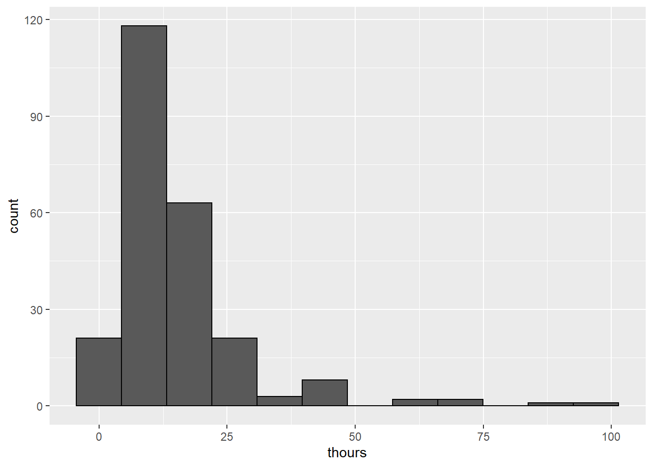
Go through our (now standard) practice of cleaning and screening the data. Examine descriptive statistics and histograms. To make things just a little easier, create a shortened dataset that contains only the following variables: admfim, disfim, thours, and episode.
IGgroup_short <- IGgroup %>%
  dplyr::select(admfim, disfim, episode, thours)

#descriptive statistics
describe(IGgroup_short)
## IGgroup_short
##
##  4  Variables      240  Observations
## --------------------------------------------------------------------------------
## admfim
##        n  missing distinct     Info     Mean      Gmd      .05      .10
##      240        0       68    0.999       68    18.44    40.00    46.00
##      .25      .50      .75      .90      .95
##    57.00    68.50    79.00    86.10    92.05
##
## lowest :  18  25  33  34  36, highest: 106 109 110 117 123
## --------------------------------------------------------------------------------
## disfim
##        n  missing distinct     Info     Mean      Gmd      .05      .10
##      240        0       74        1    85.72    22.69    47.95    55.90
##      .25      .50      .75      .90      .95
##    74.00    89.00   101.00   110.00   113.00
##
## lowest :  20  33  35  37  39, highest: 114 115 117 118 124
## --------------------------------------------------------------------------------
## episode
##        n  missing distinct     Info     Mean      Gmd      .05      .10
##      240        0       45    0.996    14.96    10.17     4.95     6.00
##      .25      .50      .75      .90      .95
##     9.00    12.00    16.00    25.00    34.05
##
## lowest :   2   3   4   5   6, highest:  67  71  79  82 100
## --------------------------------------------------------------------------------
## thours
##        n  missing distinct     Info     Mean      Gmd      .05      .10
##      240        0       42    0.998    15.12    12.04     3.00     5.00
##      .25      .50      .75      .90      .95
##     7.75    12.00    18.00    27.10    42.00
##
## lowest :  1  2  3  4  5, highest: 64 69 72 90 98
## --------------------------------------------------------------------------------
#histograms
IGgroup_short %>%
  ggplot(aes(x=thours)) +
  geom_histogram(bins=12, color = "black")
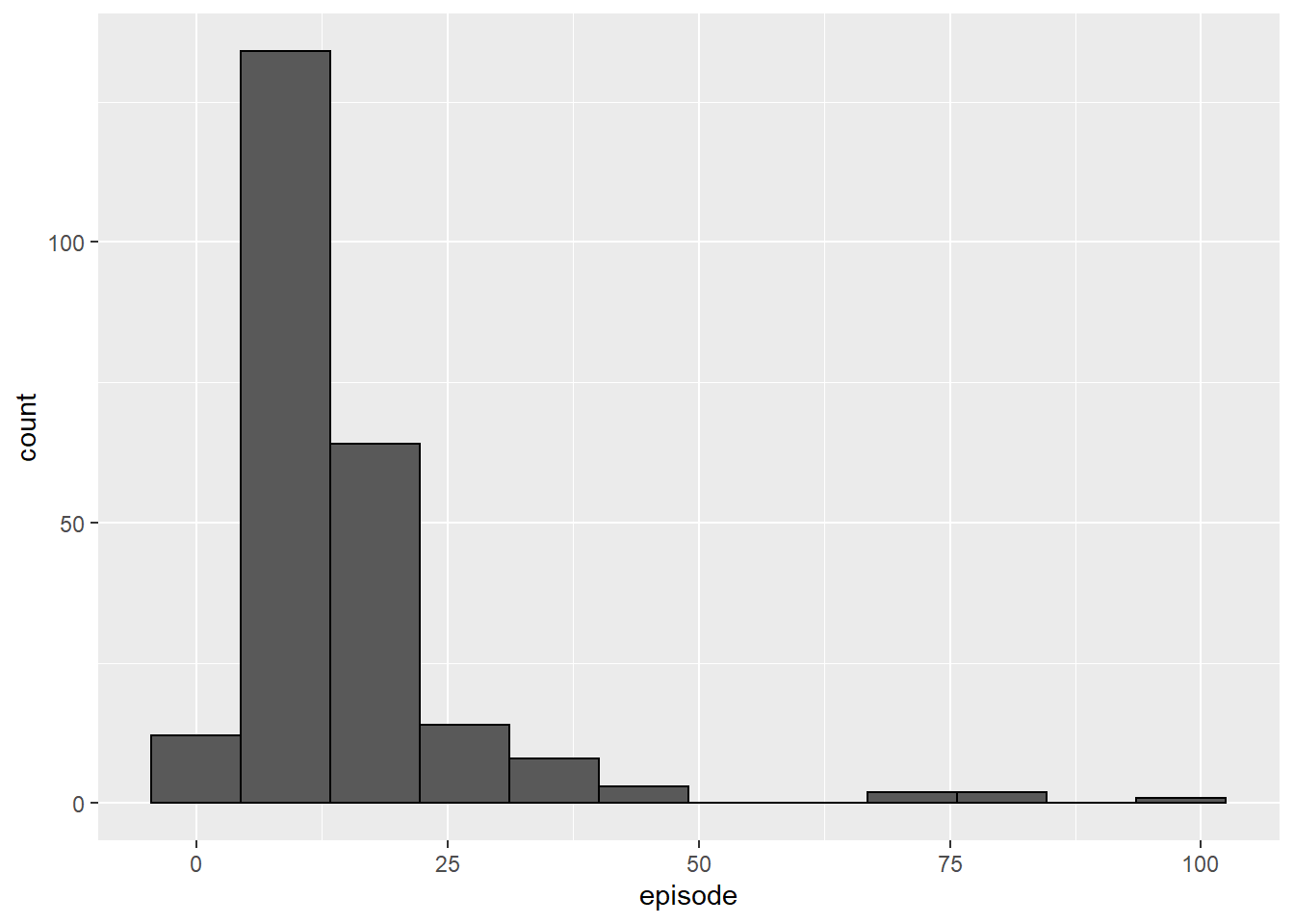
IGgroup_short %>%
  ggplot(aes(x=episode)) +
  geom_histogram(bins=12, color = "black")
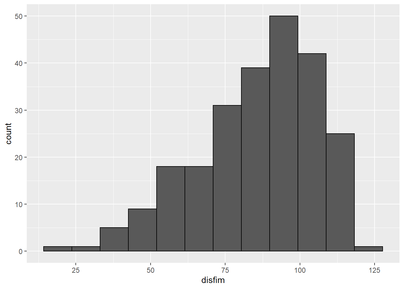
IGgroup_short %>%
  ggplot(aes(x=disfim)) +
  geom_histogram(bins=12, color = "black")
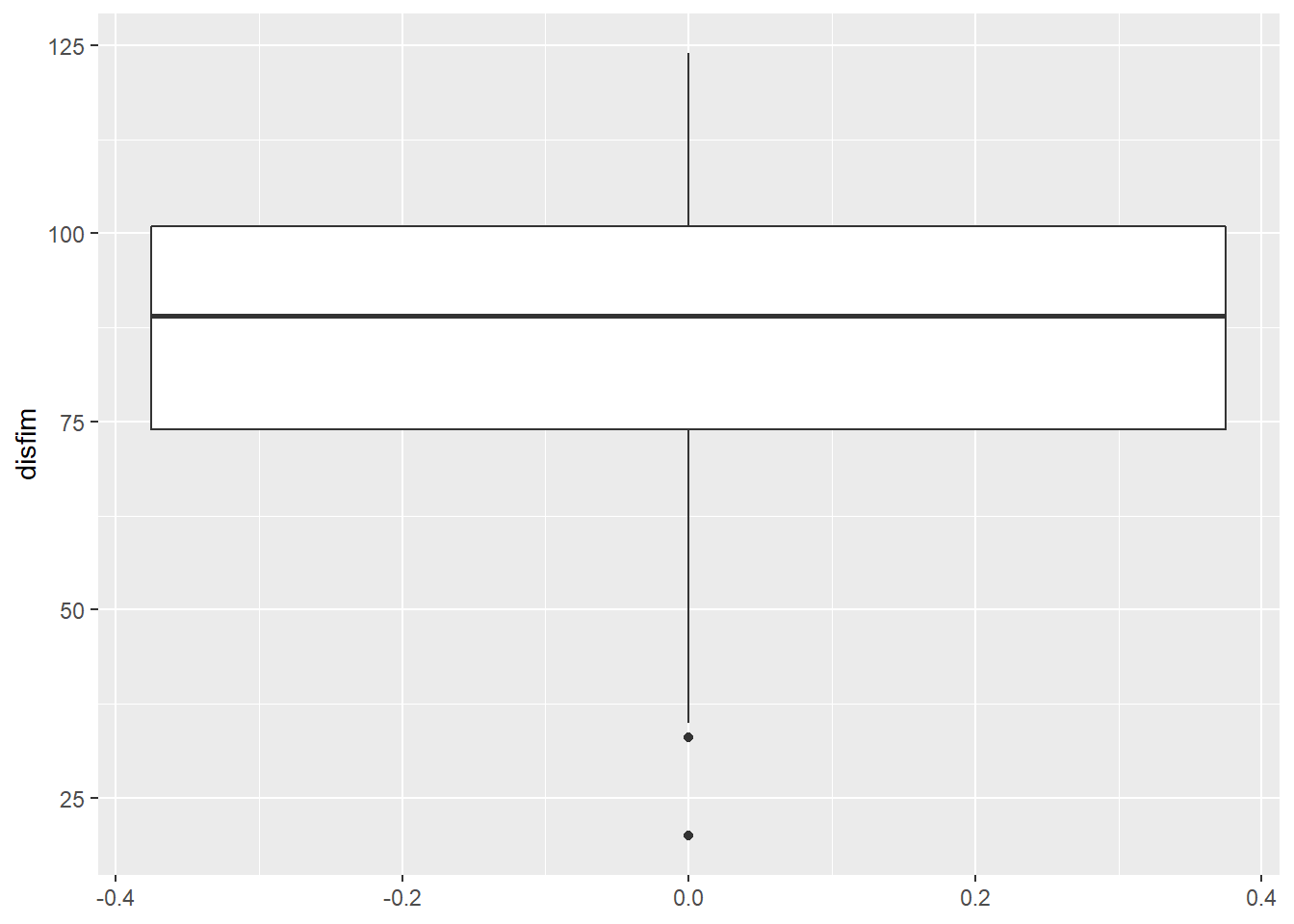
#boxplot of the dependent variable
ggplot(IGgroup_short, aes(y=disfim)) +  # This is the plot function
  geom_boxplot()
#check for outliers
IGgroup_short <- IGgroup_short %>%
  mutate(zdisfim = scale(disfim))

table(abs(IGgroup_short$zdisfim) >3.00)
##
## FALSE  TRUE
##   239     1
It looks like there is one case with a z-score greater than |3|. Because we have a large enough sample, we won’t worry about this potential outlier right now. Later on in the semester, we’ll explore how outliers can influence the regression and what to do about it.
Creating Scatterplots
Now, create scatterplots of the variables (therapy minutes versus discharge scores and length of stay versus discharge scores). Include the line of best fit.
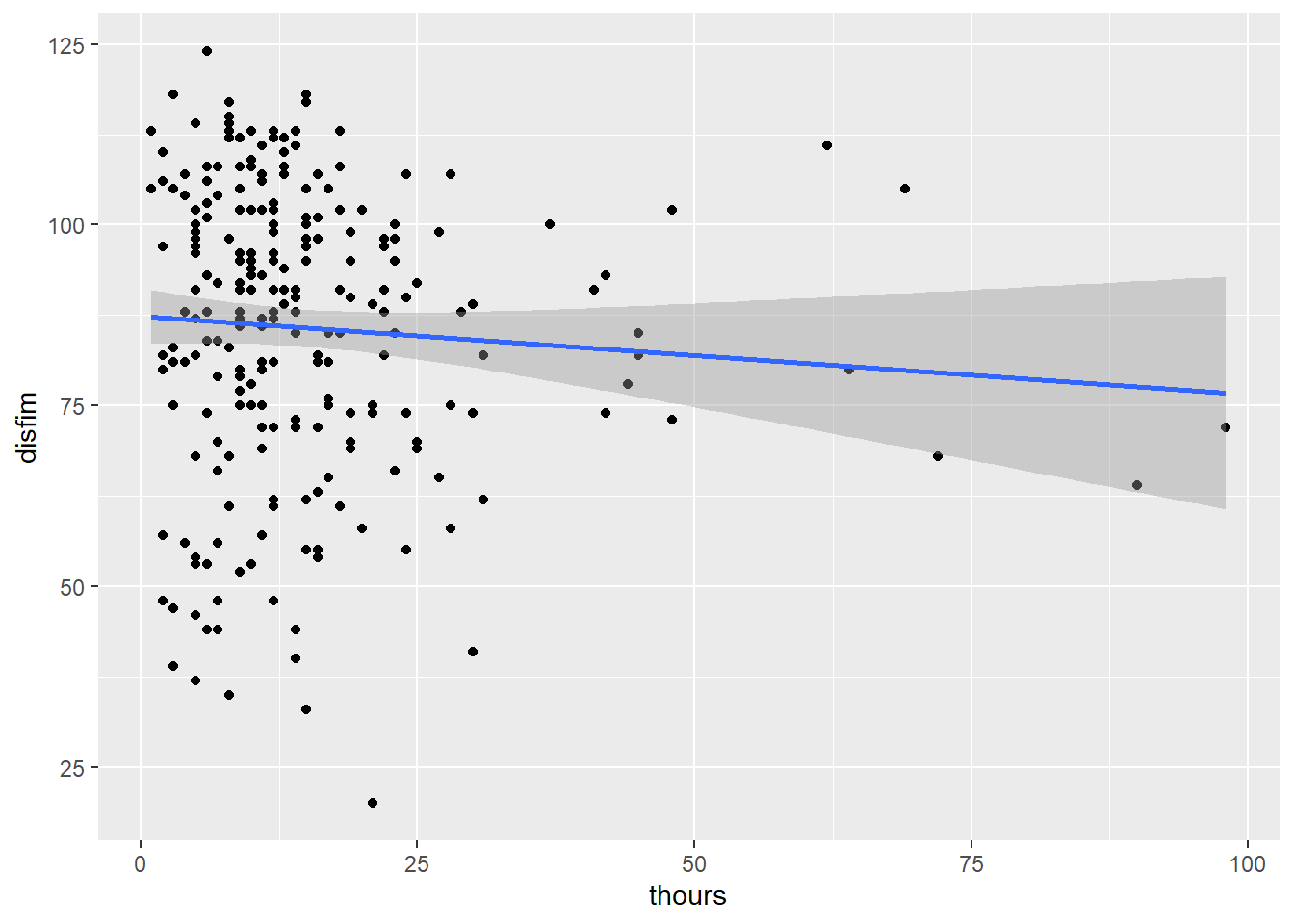
plot1 <- ggplot(IGgroup, aes(x=thours, y = disfim)) +
  geom_point() +
  geom_smooth(method="lm")
plot1
plot2 <- ggplot(IGgroup, aes(x = episode, y = disfim)) +
  geom_point() +
  geom_smooth(method = "lm")
plot2
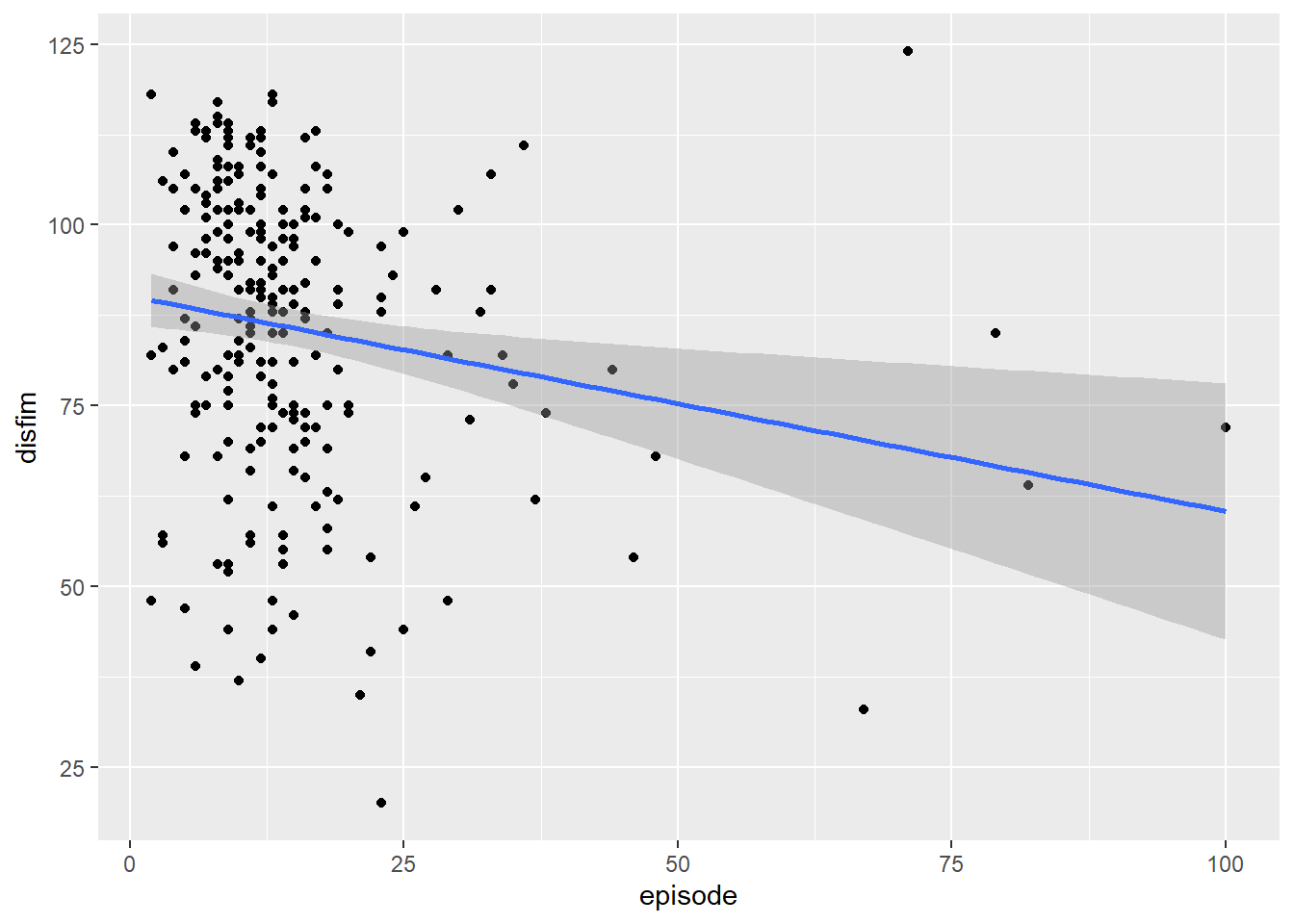
Looking at the first scatterplot between thours and disfim we can see that there is a weak negative relationship between the variables. The relationship is also negative for episode and disfim. It looks like the slope of the line for episode is slightly more negative than the line for thours.
Calculating Correlations
Let’s calculate the correlation coefficients for each pair of variables and see if the correlations line up with our conclusions based on the visualizations.
cor.test(IGgroup$thours, IGgroup$disfim)
##
## 	Pearson's product-moment correlation
##
## data:  x and y
## t = -1.1105, df = 238, p-value = 0.2679
## alternative hypothesis: true correlation is not equal to 0
## 95 percent confidence interval:
##  -0.19664113  0.05533394
## sample estimates:
##         cor
## -0.07179906
cor.test(IGgroup$episode, IGgroup$disfim)
##
## 	Pearson's product-moment correlation
##
## data:  x and y
## t = -2.8425, df = 238, p-value = 0.004865
## alternative hypothesis: true correlation is not equal to 0
## 95 percent confidence interval:
##  -0.30092522 -0.05585178
## sample estimates:
##        cor
## -0.1812002
- Interpret the correlations. Which correlation is stronger? Why?
Running the Regression Model
Now lets run our first simple regression model. The function to run regression is lm and it uses formula syntax, DV ~ IV, data = dataset. We can assign the results of the model to an object, and then call the results using summary(modelname).
therapyhrs_model <- lm(disfim ~ thours, data=IGgroup)
summary(therapyhrs_model)
##
## Call:
## lm(formula = disfim ~ thours, data = IGgroup)
##
## Residuals:
##     Min      1Q  Median      3Q     Max
## -65.089 -11.325   3.843  15.289  37.290
##
## Coefficients:
##             Estimate Std. Error t value Pr(>|t|)
## (Intercept) 87.35898    1.96465  44.465   <2e-16 ***
## thours      -0.10809    0.09733  -1.111    0.268
## ---
## Signif. codes:  0 '***' 0.001 '**' 0.01 '*' 0.05 '.' 0.1 ' ' 1
##
## Residual standard error: 20.17 on 238 degrees of freedom
## Multiple R-squared:  0.005155,	Adjusted R-squared:  0.0009751
## F-statistic: 1.233 on 1 and 238 DF,  p-value: 0.2679
How do we interpret the results of the regression model? The first line of the output is a reprint of the model that was tested. The next section contains information on the residuals. To determine if our predictor, thours is related to total discharge FIM score, we need to look at the Coefficients section. There is an estimate, a standard error, a t-value, and a p-value for each predictor in the model. The first coefficient in the model is the Intercept.
Intercept. The intercept is equal to the average FIM score for someone who received 0 hours of therapy.
Predictors. The next coefficient listed is the one for thours, which equals -0.108. For a 1-unit increase in thours (for every additional hour of therapy), there is a decrease in FIM discharge scores of .108 points.
Note that the p-value for thours is equal to the p-value for the bivariate correlation we tested above. This will always be the case when including only one predictor in the regression equation.
There are two other pieces of the output we need to examine. The Multiple R-squared, and the F-statistic.
$ R^2 $. The R-squared tells us how much variability in the dependent variable our model accounts for. In this case, because we only have one predictor, it represents how much varability thours accounts for in discharge scores. If we take the square root of $ R^2 $, we will get Pearson’s r.
F-Statistic. The F-statistic tells us if the overall model is statistically significant. In this case, the model is not significant, F(1,238) = 1.233, p = .268.
Confidence Intervals
The standard regression output does not include the 95% confidence intervals for the regression coefficients. However, we can request these by using the confint function on the saved model results.
confint(therapyhrs_model)
##                  2.5 %      97.5 %
## (Intercept) 83.4886592 91.22929860
## thours      -0.2998358  0.08365332
Standardized Regression Coefficients
The output for an lm object does not contain the standardized regression coefficients. To get those, we can use a function called lm.beta from the QuantPsyc package. Install the package if you do not already have it installed.
library(QuantPsyc)
lm.beta(therapyhrs_model)
##      thours
## -0.07179906
Note that the standardized coefficient for therapy is equal to the correlation coefficient. As with the $ R^2 $ value, this will only be true when there is one predictor in the model.
Writing out the regression equation
We can take the results of our linear regression model and write out the regression equation: $$ \hat{y}_{FIM discharge} = 87.36 -0.108*thours $$
- Now re-run the regression analysis for the other pair of variables: episode length and discharge FIM scores.
Multiple Regression
Now that you are familiar with how to run a simple regression, let’s examine a model with several predictors. This time, we’ll include both therapy hours and episode length, as well as admission FIM scores.
The process for conducting a multiple regression is pretty much identical to the process for a simple regression. Before running the model, let’s examine the correlation matrix of the 4 variables.
IGgroup %>%
  dplyr::select(admfim, disfim, episode, thours) %>%
  as.matrix() %>%
  rcorr()
##         admfim disfim episode thours
## admfim    1.00   0.79   -0.27  -0.28
## disfim    0.79   1.00   -0.18  -0.07
## episode  -0.27  -0.18    1.00   0.73
## thours   -0.28  -0.07    0.73   1.00
##
## n= 240
##
##
## P
##         admfim disfim episode thours
## admfim         0.0000 0.0000  0.0000
## disfim  0.0000        0.0049  0.2679
## episode 0.0000 0.0049         0.0000
## thours  0.0000 0.2679 0.0000
#another method: install package PerformanceAnalytics
library(PerformanceAnalytics)
IGgroup %>%
  dplyr::select(admfim, disfim, episode, thours) %>%
  chart.Correlation(., histogram=TRUE, pch=19)
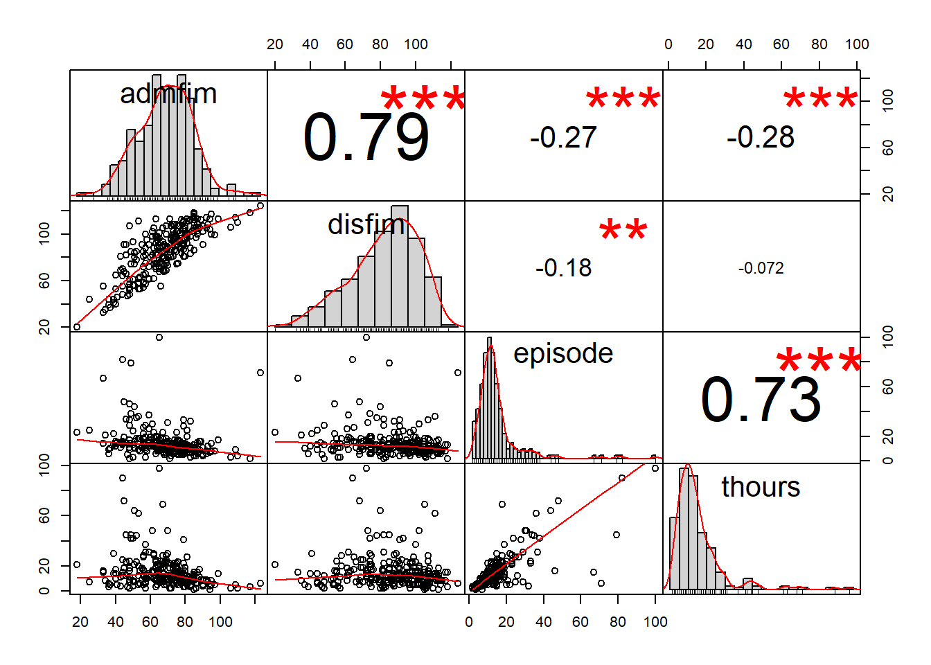
Not surprisingly, admission and discharge scores are highly correlated (.79), as are thours and episode. The remaining correlations range from -.07 to -.28.
mr_model <- lm(disfim ~ admfim + thours + episode, data= IGgroup)
summary(mr_model)
##
## Call:
## lm(formula = disfim ~ admfim + thours + episode, data = IGgroup)
##
## Residuals:
##     Min      1Q  Median      3Q     Max
## -31.602  -8.920  -0.796   7.544  42.617
##
## Coefficients:
##             Estimate Std. Error t value Pr(>|t|)
## (Intercept) 14.82134    3.81326   3.887 0.000132 ***
## admfim       1.00913    0.04871  20.719  < 2e-16 ***
## thours       0.41852    0.08425   4.968  1.3e-06 ***
## episode     -0.27032    0.09166  -2.949 0.003506 **
## ---
## Signif. codes:  0 '***' 0.001 '**' 0.01 '*' 0.05 '.' 0.1 ' ' 1
##
## Residual standard error: 11.85 on 236 degrees of freedom
## Multiple R-squared:  0.6597,	Adjusted R-squared:  0.6553
## F-statistic: 152.5 on 3 and 236 DF,  p-value: < 2.2e-16
confint(mr_model)
##                  2.5 %     97.5 %
## (Intercept)  7.3089679 22.3337073
## admfim       0.9131739  1.1050809
## thours       0.2525476  0.5844876
## episode     -0.4509006 -0.0897468
#saving the coefficients to an object to call later when writing up the results
model_mr_coefficients <- summary(mr_model)$coefficients
- Write out the regression equation for the multiple regression model.
When we control for admission scores, both therapy hours and episode length are significant predictors of FIM discharge scores. For a 1-unit increase in therapy hours, there is 0.42 point increase in FIM discharge scores, controlling for admission scores and episode length. For a 1-unit increase in episode length, there is a decrease in FIM scores of .27 points, controlling for admission scores and therapy hours.
You might have noticed that the bivariate correlation for therapy hours and FIM discharge scores was negative and non-significant. But once admission scores are partialled out, the correlation between therapy hours and discharge scores becomes positive and significant.
Admission FIM scores are a type of confounder–they are correlated with the outcome and the predictors, and so it is important to account for them in the analysis. In this example, higher admissions scores were associated with lower number of therapy hours (or, lower admissions scores were associated with higher therapy hours). Once we take that in account, we can better assess the relationship between therapy hours and discharge scores. The phenomenon of the sign changing from the bivariate relationship to the multivariate regression is referred to as supression.
In a “real” analysis, we’d likely continue exploring why the sign/significance changes to get a better understanding of what is going on with these variables. For example, we might graph the relationship between therapy hours and discharge scores for a range of admission scores to see if the relationship changes. We could also explore potential non-linear effects and interactions.
Writing up the results in APA Format
When reporting regression results in APA format, you’ll want to report both the results of the overall regression model (F with df, p-value, $ R^2 $) and the results for the predictors in the model (b or $ \beta $, SE, 95% CI, t with degrees of freedom, and p-value). If you have a several predictors, a table of the results is often easier for the reader to understand.
For the multiple regression model above:
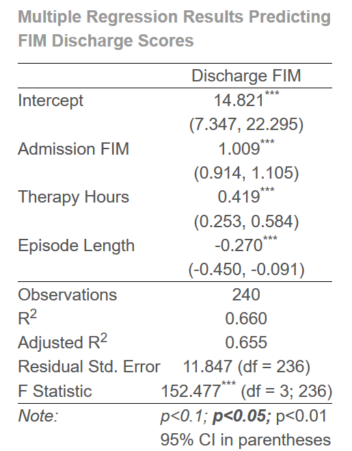
FIM discharge scores were regressed on admission FIM scores, therapy hours, and episode length. The overall regression was significant, F(3,236) = 152.48, p <.001, $ R^2 $ = .66. Admission scores were positively associated with discharge scores, b = 1.01, SE = 0.05, t(236) = 20.72, p <.001. Therapy hours were significantly and positively associated with discharge scores, b = 0.42, SE = 0.08, t(236) = 4.97, p <.001. Finally, episode length was significantly negatively associated with FIM discharge scores, b = -0.27, SE = 0.09, t(236) = -2.95, p = 0.004.
Alternative write-up:
FIM discharge scores were regressed on admission FIM scores, therapy hours, and episode length. The overall regression was significant, F(3,236) = 152.48, p <.001, $ R^2 $ = .66. All three predictors were statistically significant. Table 1 contains the a summary of the regression results. Admission scoresand therapy hours were positively associated with discharge scores,*p*s <.001, while episode length was negatively associated with discharge scores, p = 0.004.
Stargazer Package
The package stargazer creates nice regression tables and there is great documentation online for how to use the package to create well-formatted regresssion tables. You should spend some time looking at the package documentation and figuring out how to customize the tables.
results = "asis" in your chunk heading. If you are knitting to html, type = "html" should be in the code for stargazer.
library(stargazer)
stargazer(mr_model,
          title = "Multiple Regression Results Predicting FIM Discharge Scores",
          intercept.bottom = FALSE,
          covariate.labels = c("Intercept", "Admission FIM", "Therapy Hours", "Episode Length"),
          dep.var.caption = "",
          dep.var.labels = "Discharge FIM",
          type= "html",
          ci = TRUE,
          notes = "95% CI in parentheses",
          notes.append = TRUE,
          notes.align = "l")