Regression Models and Diagnostics
We will work with the neurological FIM dataset again for these exercises and limit the sample to those who are in treatment (as we did in the previous lesson). You can download the dataset here:
Download Neurological FIM Dataset
Load the dataset and subset the data so we only have those individuals who are receiving treatment:
neuro_FIM <- read_sav("neurological_FIM_Week_2.sav")

#subset the data
IGgroup_short <- neuro_FIM %>%
  subset(treatment==1) %>%
  dplyr::select(admfim, disfim, episode, thours)
In the last lesson, we used the neurological FIM dataset to examine predictors of discharge score in patients who had recieved individual + group therapy. The last model we tested was a simultaneous regression model with three predictors–admission FIM scores, therapy hours, and episode length. While this is a valid model and tells us the unique relationship between each predictor and the outcome, we aren’t that interested in the relationship between admission and discharge scores. Of course it makes sense that they are highly correlated, and it is important to include admission scores in the model. But our hypotheses are really about the effects of the other two variables–therapy hours and episode length.
Instead of a simultaneous regression model, a hierarchical model might be more appropriate in this case. We can enter admission scores in the first step of the regression which essentially controls for the variability associated with this variable. Then, we can then enter therapy hours and episode length together in the next step of the regression model. Alternatively, we could enter each variable separately on its own step. Let’s try it both ways!
Hierarchical Linear Regression
For this first example, run enter the predictors in two blocks: In the first block, enter admission FIM scores (admfim). In the second block, enter both thours and episode. You can use the update function to add the variables to the model.
#Step 1: Admission Scores
model_1 <- lm(disfim ~ admfim, data=IGgroup_short)
summary(model_1)
##
## Call:
## lm(formula = disfim ~ admfim, data = IGgroup_short)
##
## Residuals:
##     Min      1Q  Median      3Q     Max
## -28.790  -9.371  -0.080   7.687  40.629
##
## Coefficients:
##             Estimate Std. Error t value Pr(>|t|)
## (Intercept) 19.92166    3.41243   5.838 1.72e-08 ***
## admfim       0.96770    0.04878  19.838  < 2e-16 ***
## ---
## Signif. codes:  0 '***' 0.001 '**' 0.01 '*' 0.05 '.' 0.1 ' ' 1
##
## Residual standard error: 12.41 on 238 degrees of freedom
## Multiple R-squared:  0.6231,	Adjusted R-squared:  0.6216
## F-statistic: 393.6 on 1 and 238 DF,  p-value: < 2.2e-16
#Step 2:  Add thours and episode
model_2 <- update(model_1, .~. + thours + episode)
summary(model_2)
##
## Call:
## lm(formula = disfim ~ admfim + thours + episode, data = IGgroup_short)
##
## Residuals:
##     Min      1Q  Median      3Q     Max
## -31.602  -8.920  -0.796   7.544  42.617
##
## Coefficients:
##             Estimate Std. Error t value Pr(>|t|)
## (Intercept) 14.82134    3.81326   3.887 0.000132 ***
## admfim       1.00913    0.04871  20.719  < 2e-16 ***
## thours       0.41852    0.08425   4.968  1.3e-06 ***
## episode     -0.27032    0.09166  -2.949 0.003506 **
## ---
## Signif. codes:  0 '***' 0.001 '**' 0.01 '*' 0.05 '.' 0.1 ' ' 1
##
## Residual standard error: 11.85 on 236 degrees of freedom
## Multiple R-squared:  0.6597,	Adjusted R-squared:  0.6553
## F-statistic: 152.5 on 3 and 236 DF,  p-value: < 2.2e-16
So now we have the two models and we want to know how much additional variability the addition of thours and episode contributes to the model, and whether that increase in variability is statistically significant.
To calculate the change in thours and episode increased anova function to compare the two models using an F-test.
anova(model_1, model_2)
## Analysis of Variance Table
##
## Model 1: disfim ~ admfim
## Model 2: disfim ~ admfim + thours + episode
##   Res.Df   RSS Df Sum of Sq     F    Pr(>F)
## 1    238 36674
## 2    236 33121  2    3553.4 12.66 5.989e-06 ***
## ---
## Signif. codes:  0 '***' 0.001 '**' 0.01 '*' 0.05 '.' 0.1 ' ' 1
The addition of the two variables resulted in a significant increase in the variability accounted for by the model,
Now run the model and enter thours and episode in separate steps. Then compare the three models using anova.
model_3 <- update(model_1, .~. + thours)
summary(model_3)
##
## Call:
## lm(formula = disfim ~ admfim + thours, data = IGgroup_short)
##
## Residuals:
##     Min      1Q  Median      3Q     Max
## -30.836  -8.875  -0.504   7.893  39.577
##
## Coefficients:
##             Estimate Std. Error t value Pr(>|t|)
## (Intercept) 12.49859    3.79114   3.297  0.00113 **
## admfim       1.02290    0.04926  20.764  < 2e-16 ***
## thours       0.24274    0.06050   4.012 8.07e-05 ***
## ---
## Signif. codes:  0 '***' 0.001 '**' 0.01 '*' 0.05 '.' 0.1 ' ' 1
##
## Residual standard error: 12.04 on 237 degrees of freedom
## Multiple R-squared:  0.6471,	Adjusted R-squared:  0.6441
## F-statistic: 217.3 on 2 and 237 DF,  p-value: < 2.2e-16
model_4 <- update(model_3, .~. + episode)
summary(model_4)
##
## Call:
## lm(formula = disfim ~ admfim + thours + episode, data = IGgroup_short)
##
## Residuals:
##     Min      1Q  Median      3Q     Max
## -31.602  -8.920  -0.796   7.544  42.617
##
## Coefficients:
##             Estimate Std. Error t value Pr(>|t|)
## (Intercept) 14.82134    3.81326   3.887 0.000132 ***
## admfim       1.00913    0.04871  20.719  < 2e-16 ***
## thours       0.41852    0.08425   4.968  1.3e-06 ***
## episode     -0.27032    0.09166  -2.949 0.003506 **
## ---
## Signif. codes:  0 '***' 0.001 '**' 0.01 '*' 0.05 '.' 0.1 ' ' 1
##
## Residual standard error: 11.85 on 236 degrees of freedom
## Multiple R-squared:  0.6597,	Adjusted R-squared:  0.6553
## F-statistic: 152.5 on 3 and 236 DF,  p-value: < 2.2e-16
anova(model_1, model_3, model_4)
## Analysis of Variance Table
##
## Model 1: disfim ~ admfim
## Model 2: disfim ~ admfim + thours
## Model 3: disfim ~ admfim + thours + episode
##   Res.Df   RSS Df Sum of Sq       F   Pr(>F)
## 1    238 36674
## 2    237 34342  1    2332.7 16.6215 6.24e-05 ***
## 3    236 33121  1    1220.7  8.6977 0.003506 **
## ---
## Signif. codes:  0 '***' 0.001 '**' 0.01 '*' 0.05 '.' 0.1 ' ' 1
Each additional step accounted for significant variability in the model, as indicated by the ANOVA results.
- Calculate the change in
Regression Diagnostics
This week, we are introducing some new data cleaning and screening procedures that you should incorporate into your analysis habits. In addition to examining the descriptive statistics and histograms/boxplots, we’ll also now need to look for outliers and influential cases. Your data cleaning/screening process should now go through the following steps:
Check for accuracy. Make sure that scores for each variable are in the expected range. Correct or delete cases with out of range values.
Assess missing data. Although we aren’t covering missing data in this course, you should know how much you have; less than 5% missing per variable is not usually a problem; more than that and you need to think about imputation or estimation techniques like maximum likelihood that can take missing data into account)
Run Descriptives and Visualizations. Examine the descriptive statistics and distributions of your variables, and in particular, the dependent variable.
Check for univariate and multivariate outliers. Use z-scores to check for univariate outliers and Mahalanobis distance to check for multivariate outliers. Outliers are not always a problem–with large sample sizes, a few outliers are okay and even expected (there will be scores in the tails, but you shouldn’t have more than 2.5% in either direction). For multivariate outliers, consider removing cases if they also are extreme on other influence measures (Cooks, leverage–see below).
Examine influence statistics. Check for cases that exceed cut-offs for Cook’s distance and leverage, indicating highly influential cases. If cases are extreme on two or more outlier/influence measure (Mahalanobis, Cooks, Leverage), consider removing them from the analysis.
Examine multicollinearity. Run correlations on the variables included in the model. Correlations between predictors should not exceed .90, but can be problematic at .70 or above. Predictors should be correlated with the outcome variable.
Check Assumptions of the GLM.
- Linearity/Additivity: Scatterplots, Q-Q plot
- Normality of the residuals: Histogram of the standardized residuals
- Homogeneity of variances/Homoscadasticity: Plot standardized residuals against predicted values; plot should look like a blob (no fanning or butterfly shape)
Mahalanobis Distance, Leverage, and Cook’s Distances
Last week, we ran descriptives and visualizations of our variables so there is no need to redo that here. Instead, we’ll skip right to examining/identifying outliers and influential cases.
Although it seems a bit counterintuitive, we actually need to run the regression model first in order to then calculate/examine the outliers/influential cases. We’ll need to run the final model–the one that contains all of our variables. We did this last week. If you still have the model in your environment, great! If not, run it again and make sure to save the results to an object.
final_model <- lm(disfim ~ admfim + thours + episode, data=IGgroup_short)
We’ll start with Mahalanobis distance. You should not run this function on a dataset that includes categorical variables. You can tell R to exclude the ID column and any categorical columns using datasetname[,-1], replacing the -1 with the column number or numbers you want to exclude. This code would exclude the first column of the dataset (so you can adapt it for your own purposes). To make things a little easier for this example, we will use the IGgroup_short dataset that only contains the variables included in our final model.
First, calculate the mahalanobis distances for each case using the mahalanobis function. Then, calculate and save the cut-off value. The cut-off value is based on a chi-square distribution with degrees of freedom equal to the number of variables included in the analysis. We want to know if values exceed a threshold of p<.001 (i.e., more extreme than .001).
We can then create a table that tells us how many cases in the dataset have “bad” mahalanobis values.
mahal = mahalanobis(IGgroup_short,
                    colMeans(IGgroup_short),
                    cov(IGgroup_short))

mahal_cutoff = qchisq(1-.001, ncol(IGgroup_short))
badmahal = as.numeric(mahal > mahal_cutoff)
table(badmahal)
## badmahal
##   0   1
## 232   8
Leverage values are saved as part of the standard output when running a lm model and called hatvalues. We will resave these values to a new object called leverage.
The cut-off value for leverage is: \(\frac{2*k+2}{N}\).k is equal to the number of predictors in the final step of the regression model (i.e., the final model). We then create a table that shows us how many cases have a “bad” leverage value.
##leverage
k = 3 ##number of IVs in the final step
leverage = hatvalues(final_model)
cutleverage = (2*k+2) / nrow(IGgroup_short)
badleverage = as.numeric(leverage > cutleverage)
table(badleverage)
## badleverage
##   0   1
## 224  16
We can use the cooks.distance function to get the cook’s values for each case in the dataset. We then need to calculate the cut-off score, which is equal to:
##cooks
cooks = cooks.distance(final_model)
cutcooks = 4 / (nrow(IGgroup_short) - k - 1)
cutcooks ##get the cut off
## [1] 0.01694915
badcooks = as.numeric(cooks > cutcooks)
table(badcooks)
## badcooks
##   0   1
## 229  11
In total, 7 cases have bad Mahalanobis scores, 16 have bad leverage scores, and 11 have bad cook’s scores. What should we do with this information? Having one bad score on any of these three measures is not necessarily problematic. It may be more of a problem if a case is bad on two or three of these measures.
For each measure we calculated above, we saved a variable that tells us whether case is good or bad (0 for okay, 1 for bad). We can sum across these three variables, creating a variable that represents the number of times a case was bad cases on mahalanobis, leverage, and cooks.
##overall outliers
##add them up!
totalout = badmahal + badleverage + badcooks
table(totalout)
## totalout
##   0   1   2   3
## 220   9   7   4
Based on the table we get, there are a total of 11 cases that have 2 or 3 bad values. Our next decision is whether to exclude these cases or not. My personal opinion on removing cases from a dataset is that the decision should be based on more than just the numbers. Is there something about the case(s) that suggests this person is not a member of the population I am trying to sample from? Are the values, and combinations of those values, realistic? If the answer to those questions is “NO”, then go ahead and remove them.
Another strategy is to run the models with and without those cases included. If removing the cases doesn’t change the overall story of the results, Yay! Leave them in. If it does change the story, then you have some decision to make. You can proceed with excluding the cases and explain in your write up why you did so. Another strategy would be to use robust regression. In general, robust regression analyses do not make the same assumptions as the general linear model, and can be a good strategy to employ when you encounter problematic data. However, there are tons of different robust regression procedures that can be implemented in R, and different robust packages use different procedures and different default settings when running the analysis. If you decide to use robust regression, you’ll want to do some research on what type of analysis is most appropriate and pick a package in R that best meets your needs. Later in this exercise, we’ll run the model using robust regression from the robustbase package.
Just for practice, create a new dataset that excludes cases that have 2 or more bad outlier scores. Then re-run the regression model. Load the car library and then use the compareCoefficients function to examine the differences in the coefficients between our original model and the model removing outliers.
IGgroup_noout <- subset(IGgroup_short, totalout <2)

model_noout <- lm(disfim ~ admfim + thours + episode, data=IGgroup_noout)
summary(final_model)
##
## Call:
## lm(formula = disfim ~ admfim + thours + episode, data = IGgroup_short)
##
## Residuals:
##     Min      1Q  Median      3Q     Max
## -31.602  -8.920  -0.796   7.544  42.617
##
## Coefficients:
##             Estimate Std. Error t value Pr(>|t|)
## (Intercept) 14.82134    3.81326   3.887 0.000132 ***
## admfim       1.00913    0.04871  20.719  < 2e-16 ***
## thours       0.41852    0.08425   4.968  1.3e-06 ***
## episode     -0.27032    0.09166  -2.949 0.003506 **
## ---
## Signif. codes:  0 '***' 0.001 '**' 0.01 '*' 0.05 '.' 0.1 ' ' 1
##
## Residual standard error: 11.85 on 236 degrees of freedom
## Multiple R-squared:  0.6597,	Adjusted R-squared:  0.6553
## F-statistic: 152.5 on 3 and 236 DF,  p-value: < 2.2e-16
summary(model_noout)
##
## Call:
## lm(formula = disfim ~ admfim + thours + episode, data = IGgroup_noout)
##
## Residuals:
##     Min      1Q  Median      3Q     Max
## -32.985  -8.474  -0.657   7.478  40.951
##
## Coefficients:
##             Estimate Std. Error t value Pr(>|t|)
## (Intercept) 11.41104    4.46040   2.558   0.0112 *
## admfim       1.03422    0.05303  19.503  < 2e-16 ***
## thours       0.51252    0.11981   4.278 2.79e-05 ***
## episode     -0.22138    0.15914  -1.391   0.1656
## ---
## Signif. codes:  0 '***' 0.001 '**' 0.01 '*' 0.05 '.' 0.1 ' ' 1
##
## Residual standard error: 11.51 on 225 degrees of freedom
## Multiple R-squared:  0.6515,	Adjusted R-squared:  0.6469
## F-statistic: 140.2 on 3 and 225 DF,  p-value: < 2.2e-16
#compare the coefficients from the model using the full dataset versus outliers removed
compareCoefs(final_model, model_noout)
## Calls:
## 1: lm(formula = disfim ~ admfim + thours + episode, data = IGgroup_short)
## 2: lm(formula = disfim ~ admfim + thours + episode, data = IGgroup_noout)
##
##             Model 1 Model 2
## (Intercept)   14.82   11.41
## SE             3.81    4.46
##
## admfim       1.0091  1.0342
## SE           0.0487  0.0530
##
## thours       0.4185  0.5125
## SE           0.0842  0.1198
##
## episode     -0.2703 -0.2214
## SE           0.0917  0.1591
##
- After comparing the two analyses, what do you conclude?
Checking Assumptions
In addition to outliers, we also need to check that we have not violated any assumptions of the general linear model. Last week, we ran correlations between the variables and saw that there were a couple high correlations of about .70. We have multicollinearity in the dataset, but we should check to see if it is a big problem by examining the VIF and tolerance statistics. Ideally, we do not want the VIF to exceed 10 (or 4, if we want to be conservative), and we would also like the average VIF across the predictors to be less than 1.
vif(final_model)
##   admfim   thours  episode
## 1.094653 2.171483 2.155352
None of the VIF exceed 4 (or 10), but if we were to average across them, we would get a value larger than 1. We can probably keep all of the variables in the model, although we might consider removing one of them to reduce the collinearity in the model.
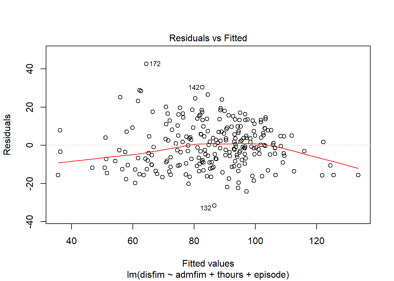
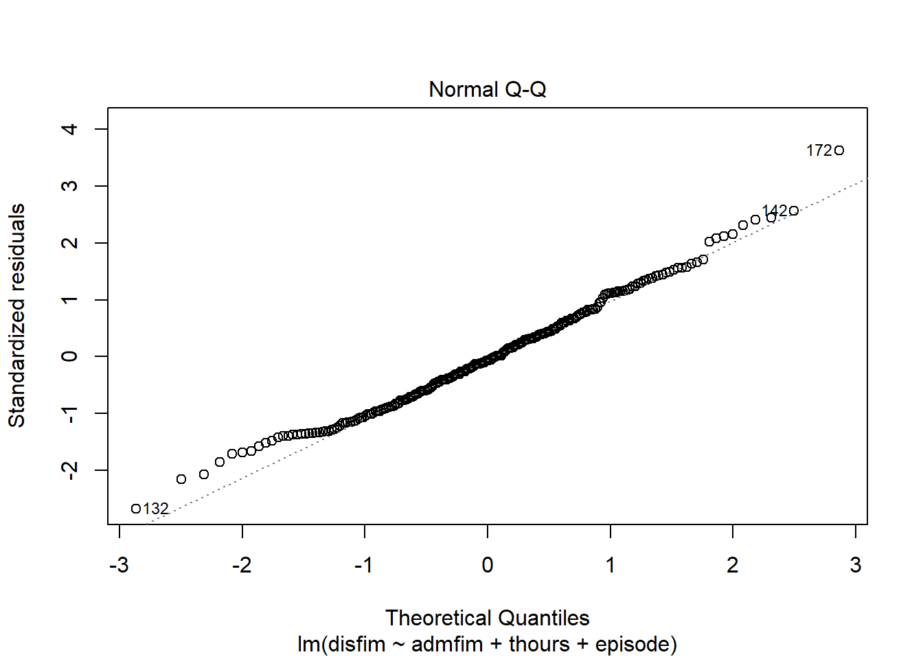
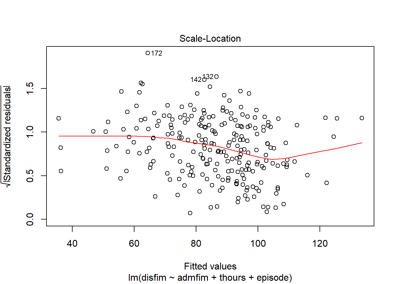
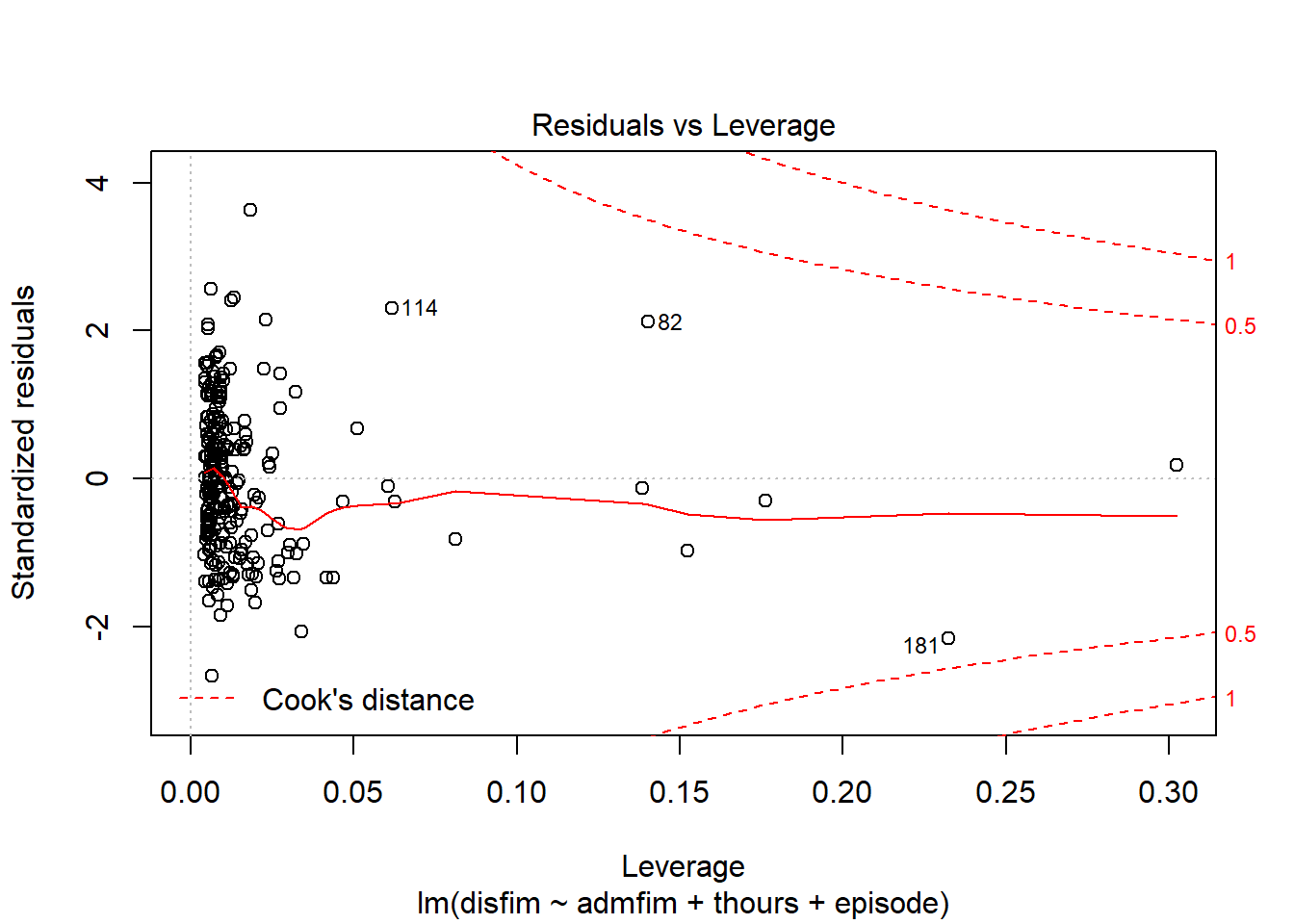
Plots of the residuals
We can use the plot function on the model we tested to examine a number of diagnostic plots. By default, we will get 4 different plots: (1) residuals versus fitted values, (2)q-q plot, (3)square root of residuals v fitted values, and (4) residuals versus leverage.
#using the plot function:
plot(final_model)
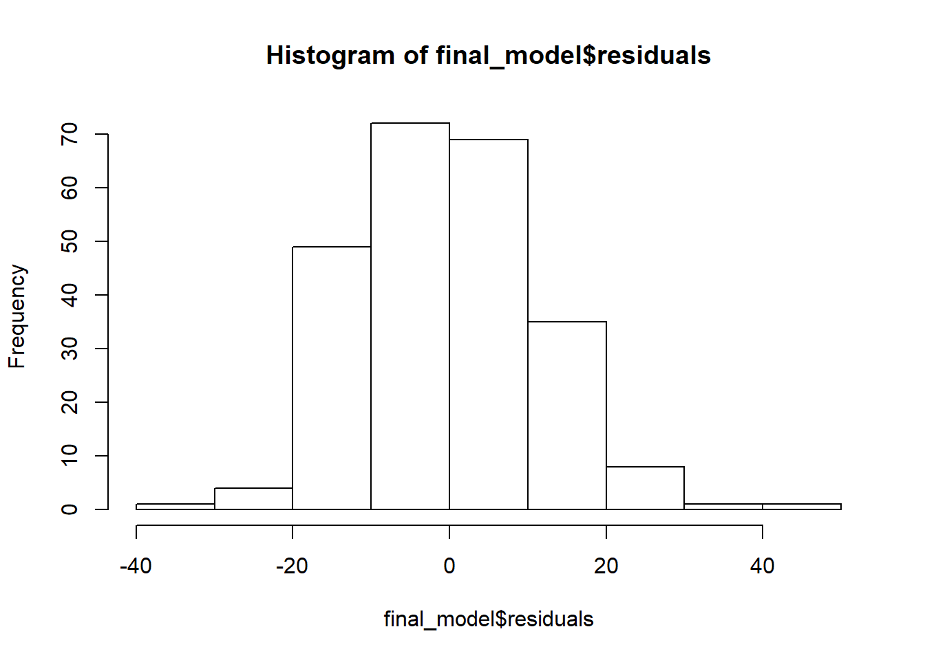
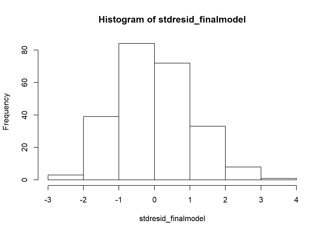
If we want to get a histogram of the standardize residuals, we will need to use the rstandard function on the residuals of the model. Then we can use the hist function to create the histogram.
#plotting the residuals from the model
hist(final_model$residuals)
#saving the standardized residuals to an object, then plotting histogram
stdresid_finalmodel <- rstandard(final_model)
hist(stdresid_finalmodel)
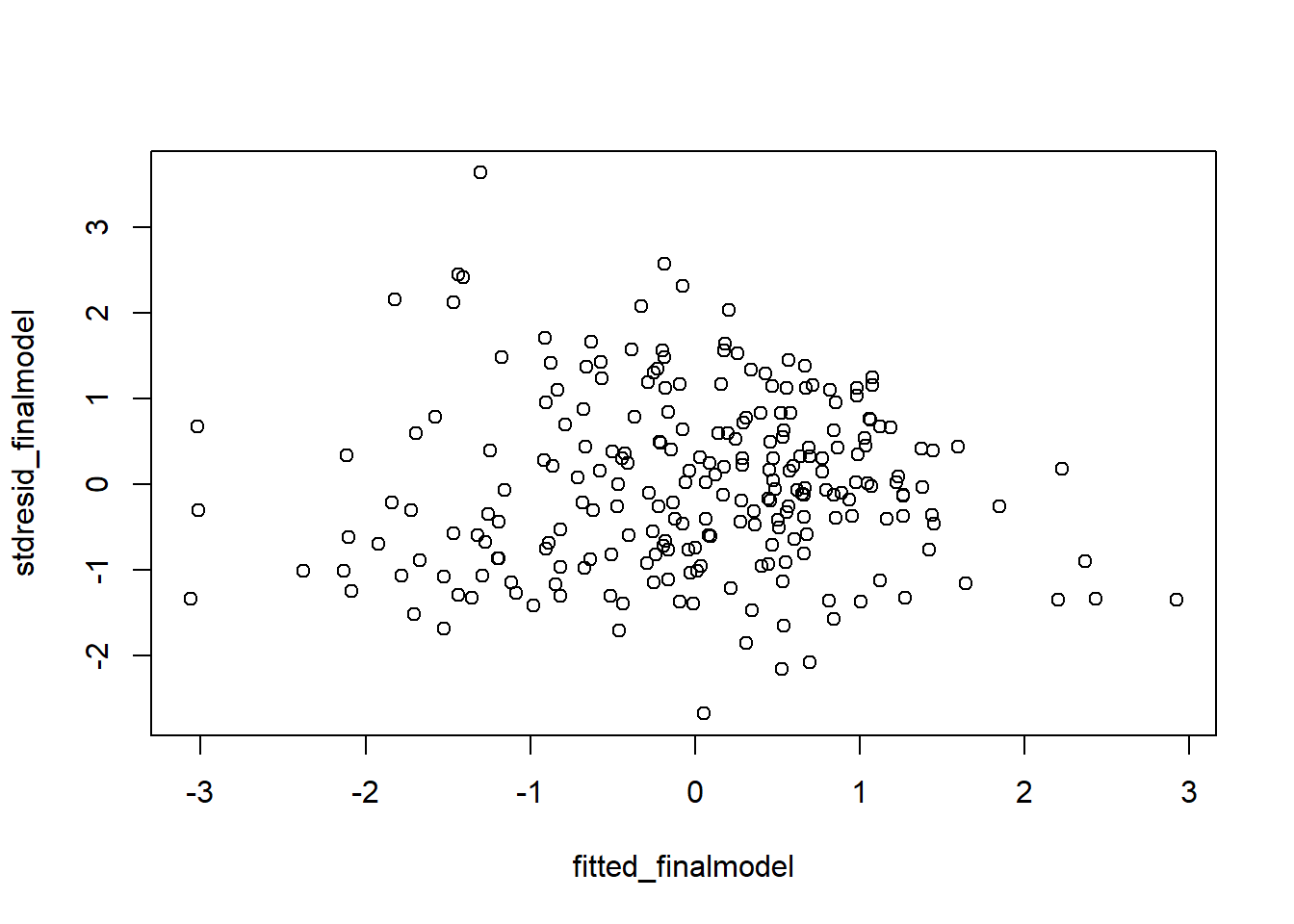
Although the plot function we used above on the model gave us a plot of the residuals versus fitted, it is better to look at the standardized version of that plot. We aleady saved the standardized residuals above, so we just need to get standardized fitted values and then run the plot:
#plot of standardized residuals versus standardized fitted values
fitted_finalmodel <- scale(final_model$fitted.values)
plot(fitted_finalmodel, stdresid_finalmodel)
car Package Regression Diagnostics
The car package has a number of functions that you can call that perform various regression diagnostics.
#set of residual plots
residualPlots(final_model)
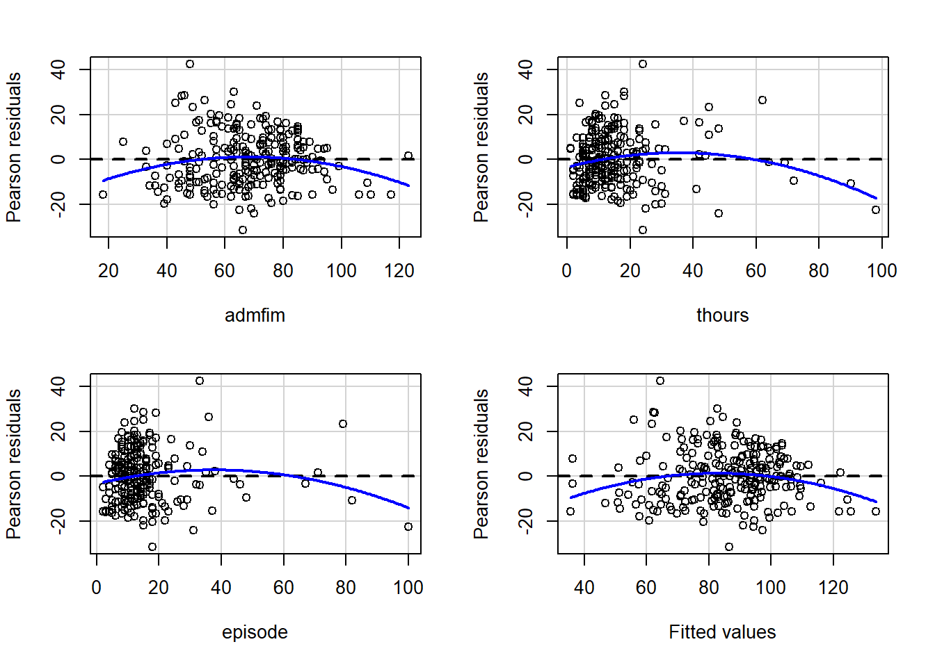
##            Test stat Pr(>|Test stat|)
## admfim       -2.5005         0.013084 *
## thours       -2.8460         0.004819 **
## episode      -2.1997         0.028803 *
## Tukey test   -2.8050         0.005031 **
## ---
## Signif. codes:  0 '***' 0.001 '**' 0.01 '*' 0.05 '.' 0.1 ' ' 1
#qq Plots
qqPlot(final_model)
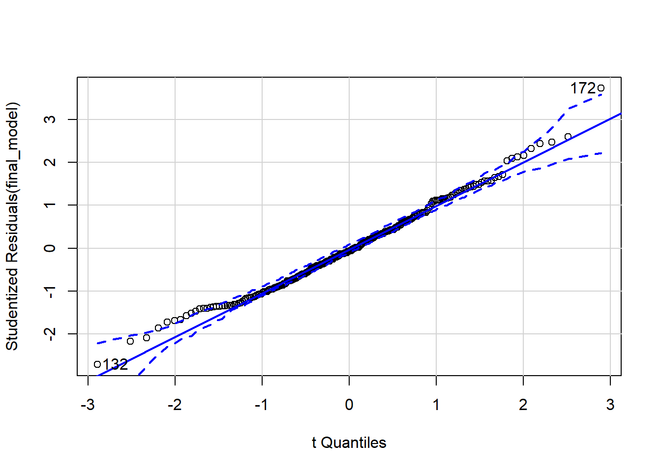
## [1] 132 172
#Tests for outliers based on studentized residuals
outlierTest(final_model)
## No Studentized residuals with Bonferroni p < 0.05
## Largest |rstudent|:
##     rstudent unadjusted p-value Bonferroni p
## 172 3.728865         0.00024111     0.057867
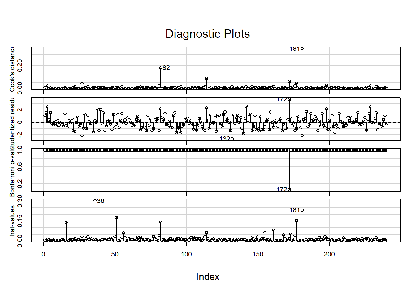
#Influence plots including Cook's distance and leverage
influenceIndexPlot(final_model)
#Bubble plt of residuals, leverage, and cook's
influencePlot(final_model)
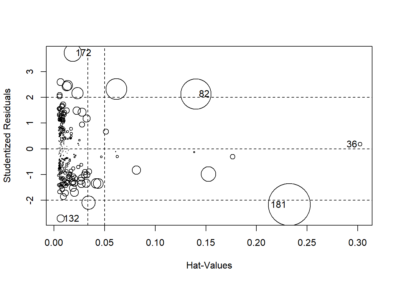
##        StudRes         Hat       CookD
## 36   0.1752673 0.302321284 0.003341506
## 82   2.1328314 0.140267479 0.182795041
## 132 -2.7121388 0.006504534 0.011723920
## 172  3.7288654 0.018389973 0.061746862
## 181 -2.1749924 0.232489114 0.352664788
#non-constant error variance
test.episode <- ncvTest(model_noout, ~episode)
test.episode
## Non-constant Variance Score Test
## Variance formula: ~ episode
## Chisquare = 3.955657, Df = 1, p = 0.046714
test.thours <-ncvTest(model_noout, ~thours)
test.thours
## Non-constant Variance Score Test
## Variance formula: ~ thours
## Chisquare = 3.08486, Df = 1, p = 0.079024
test.both <- ncvTest(model_noout, ~thours + episode)
test.both
## Non-constant Variance Score Test
## Variance formula: ~ thours + episode
## Chisquare = 4.169212, Df = 2, p = 0.12436
test.model <- ncvTest(model_noout)
test.model
## Non-constant Variance Score Test
## Variance formula: ~ fitted.values
## Chisquare = 8.271164, Df = 1, p = 0.004028
Effect sizes: Partial Correlations
The standardized coefficient (
Another effect size you can use for linear regression predictors is the partial correlation, ppcor package to calculate partial correlations. We can use that package again here to calculate the partial correlations for each of our predictors. We’ll then need to square the partial correlations to get
squared_partials <- (pcor(IGgroup_short, method="pearson")$estimate)^2
squared_partials
##              admfim     disfim     episode     thours
## admfim  1.000000000 0.64525771 0.009096138 0.10244153
## disfim  0.645257713 1.00000000 0.035544779 0.09467249
## episode 0.009096138 0.03554478 1.000000000 0.51709924
## thours  0.102441533 0.09467249 0.517099237 1.00000000
- What are the
Robust Regression
Make sure you do the robust regression on the right dataset–we want to use the dataset that includes all of the cases (not the one where we removed the outliers).
Install the robustbase package and then load the library. The code for running robust regression is nearly identical to that for linear regression. Just change the lm to lmrob.
library(robustbase)
robust_model <- lmrob(disfim ~ admfim + thours + episode, data=IGgroup_short)
summary(robust_model)
##
## Call:
## lmrob(formula = disfim ~ admfim + thours + episode, data = IGgroup_short)
##  \--> method = "MM"
## Residuals:
##      Min       1Q   Median       3Q      Max
## -31.2336  -8.3341  -0.6188   7.8240  44.3213
##
## Coefficients:
##             Estimate Std. Error t value Pr(>|t|)
## (Intercept) 11.71449    4.75873   2.462  0.01455 *
## admfim       1.04906    0.05548  18.910  < 2e-16 ***
## thours       0.45363    0.08406   5.397 1.65e-07 ***
## episode     -0.31145    0.09395  -3.315  0.00106 **
## ---
## Signif. codes:  0 '***' 0.001 '**' 0.01 '*' 0.05 '.' 0.1 ' ' 1
##
## Robust residual standard error: 11.38
## Multiple R-squared:  0.6828,	Adjusted R-squared:  0.6787
## Convergence in 14 IRWLS iterations
##
## Robustness weights:
##  19 weights are ~= 1. The remaining 221 ones are summarized as
##    Min. 1st Qu.  Median    Mean 3rd Qu.    Max.
## 0.09515 0.86500 0.94420 0.90250 0.98310 0.99900
## Algorithmic parameters:
##        tuning.chi                bb        tuning.psi        refine.tol
##         1.548e+00         5.000e-01         4.685e+00         1.000e-07
##           rel.tol         scale.tol         solve.tol       eps.outlier
##         1.000e-07         1.000e-10         1.000e-07         4.167e-04
##             eps.x warn.limit.reject warn.limit.meanrw
##         2.237e-10         5.000e-01         5.000e-01
##      nResample         max.it       best.r.s       k.fast.s          k.max
##            500             50              2              1            200
##    maxit.scale      trace.lev            mts     compute.rd fast.s.large.n
##            200              0           1000              0           2000
##                   psi           subsampling                   cov
##            "bisquare"         "nonsingular"         ".vcov.avar1"
## compute.outlier.stats
##                  "SM"
## seed : int(0)